Hidden Geometry of Large Language Models

This post is based on a paper with Jiajun Song.

Can we trust Large Language Models?

If you are reading this blog, most probably you know what ChatGPT is. “How fascinating!” You may exclaim. Yes, it is indeed magical to interact with a chatbot that seemingly understand our languages. The more we play with ChatGPT, the more surprises we have: it is super knowledgeable, good at drafting emails, polishing essays, writing codes, and so on!

But then wait … when you give elementary-level mathematical questions—as simple as multiplication—as prompts, it sometimes outputs wrong solutions. There are many pitfuls: LLMs often hallucinate, and they cannot infer basic relations such as “A is B” implying “B is A” . So we ask—

• Can we trust ChatGPT as well as other Large Lauguage Models (LLMs)?
• Is it possible that LLMs contain harmful information or bias?
• Shouldn’t we worry that LLMs may distort information and influence people’s opinons?

Indeed, if our future society depends heavily on an advancing technology, there are good reasons to be concerned about the worst case scenarios (think about industrial revoluation and global warming).

There are now heated discussions about ChatGPT. AI leaders such as Yoshua Bengio, Geoffrey Hinton, Andrew Yao are calling for safe AI systems in a recent post.

Towards mechanistic explanation

Reflecting on history: Emergence of black-box models

When I first took courses in data analysis as an undergrad about a decade ago, every method is based on principled generative models: assuming that our data follow a linear model with observational noise, then we know how to extract signals from data, often in an optimal way. Moreover, we reasonably believe that data usually possess nice geometric structures, such as smoothness and sparsity. Principled mathematical analysis leads to ubiquitous methods such as LASSO and compressed sensing.

However, when data are very complex—think about images, audios, texts—we are limited by our abilities to model the data precisely. An early neural network model, AlexNet, shows that large models with multiple layers are very efficient at capturing nonlinearity. This marks the beginning of the deep learning revolutionary.

Neural networks as black-box models are highly accurate, yet much less interpretable. Lack of interpretability is a persistent and crucial issue in LLMs, as people build larger and larger models based on modules we don’t quite understand.

Visualizing attention matrix

Since the Attention is all you need paper, Transformers become the de facto building blocks of LLMs. Sometimes we can peep inside the model by plotting the attention matrices, which suggest how information of words in a sequence is combined. Mathematical speaking, given embeddings (or hidden states) \(\boldsymbol{x}_1 \ldots \boldsymbol{x}_T \in \mathbb{R}^d\), we stack them into a matrix \(\boldsymbol{X} = [\boldsymbol{x}_1, \ldots, \boldsymbol{x}_T]^\top \in \mathbb{R}^{T \times d}\) and compute a \(T \times T\) attention matrix

\[\begin{equation} \boldsymbol{A} = \mathrm{softmax}\left(\frac{\boldsymbol{X} \boldsymbol{W}^q (\boldsymbol{W}^k)^\top \boldsymbol{X}^\top}{\sqrt{d_{\mathrm{head}}}} \right)\, . \tag{1} \label{attn} \end{equation}\]

Here, \(d_{\mathrm{head}}\) is some dimension, \(\boldsymbol{W}^q\) and \(\boldsymbol{W}^k\) are trained weights in transformers, and \(\mathrm{softmax}\) applies the standard softmax

\[\begin{aligned} \left( \mathrm{softmax}(\boldsymbol{z}) \right)_{k} := \frac{e^{z_k}}{\sum_{j} e^{z_j}}, \qquad \text{where}~\boldsymbol{z} \in \mathbb{R}^T \end{aligned}\]

to every row vector of the matrix inside the paranthesis. For a given input sequence, visualizing the attention matrices (there are many in a transformer!) helps us to understand how information is processed. For example, I pass some random sequence to GPT-2, and examine the associated attention matrix \(\boldsymbol{A}\) from layer 5, head 1. It is worthwhile to note that many GPT-style transformers (including chatGPT!) are based on next-token prediction, so each token is only allowed to attend to past tokens in a sequence. Below I can use separate heatmaps (left) to visualize three selected attention matrices (Layer 0, Head 1; Layer 2, Head 2; Layer 5, Head 1), and overlapping three bipartite graphs (right) to visualize the same three matrices.

On the right side of the bipartite graph, each token is connected to tokens on the left. The thicker a line is, the more information we assemble to form the hidden states in the next layer. For example, the red lines (based on one attention matrix) mean that a token prefers to focus on the previous token.

Interpretability: some recent progress

Anthropic pinoneers Mechanistic Interpretability of neural networks, in which weights and activations are examined and analyzed closely. By studying transformers and extensive experiments, they identified that an interesting component, called the induction head, exists universally in popular trained transformered

Induction Head is a circuit—often a collection of several attention heads—within a transformer than functions the copying mechanism: given a sequence that contains tokens [A], [B] … [A], an induction head outputs values that leads to predicting [B]. In other words, induction heads complete an observed pattern by looking at the previous tokens in a sequence.

A surprising phenomenon is that induction heads function as copying mechanisms even when [A], [B] are drawn from distributions that are totally different from training data! In Figure \ref{attn}, we already saw an exmaple of induction head: once observing [A], [B] … [A], the attention heads focus heavily on the adjacent token [B] of the previous identical token [A]. Note that the input sequence is a repetition of independent random tokens, yet GPT-2 is trained on natural languages.

The above GIF highlights what each token attends to in the three attention heads as in Figure \ref{attn}.

Analyzing abstract abilities like induction heads in trained transformers opens the door to understanding in-context learning and other emergent abilities of LLMs. The more we understand, the better we are at reining in LLMs before large AI sysmtems wreak havoc!

From heuristics to uncovering hidden geometry

When people build new neural network architectures or devise new optimization tricks, they often rely on heuristics which vaguely describe the information some activations or weights contain. For example, transformers consist of many self-attention layers, each of which is believed to contextualize features progressively, i.e., combining information within contexts to form high-level features.

If we examine the arguments people make in the literature, an implicit and recurring assumption seems to be the following:

Hidden states (or activations) in intermediate layers of transformers carry certain information about input sequence contexts, and certain information about token positions.

Can we understand more precisely what information hidden states contain?

ANOVA-inspired decomposition

Suppose that we are given an input sequence, where each token has an embedding, that is, representation by numerical values \(\boldsymbol{h_t}^{(0)} \in \mathbb{R}^d\) where \(t\) is an integer indicating the position of the token. Let us write each layer of a transformer as \(\mathrm{TFLayer}_\ell\), which maps a sequence of hidden states to another for a given initial embeddings \(\boldsymbol{h}_1^{(\ell)}, \ldots, \boldsymbol{h}_T^{(\ell)} \in \mathbb{R}^d\):

\[\begin{aligned} \boldsymbol{h}_1^{(\ell+1)}, \ldots, \boldsymbol{h}_T^{(\ell+1)} \leftarrow \mathrm{TFLayer}_\ell \left( \boldsymbol{h}_1^{(\ell)}, \ldots, \boldsymbol{h}_T^{(\ell)} \right) \end{aligned}\]

Let’s sample as many sequences as we want, feed each sequence through a trained transformer, and collect all these hidden states (or intermediate-layer embeddings) as an array \(\boldsymbol{h}^(\ell) \in \mathbb{R}^{C \times T \times d}\). Here \(C\) is the number of sequences we sample, \(T\) is the sequence length, and \(d\) is the dimension of hidden states.

A classical idea in statistics, known as ANOVA, is to study the mean effects of each factor in a collection of observations. Based on \(\boldsymbol{h}^{(\ell)}\), we can calculate the mean vectors for every position and for every input sequence.

\[\begin{aligned} \boldsymbol{pos}_t^{(\ell)} := \frac{1}{C} \sum_{c=1}^C \boldsymbol{h}_{t,c}^{(\ell)} - \boldsymbol{\mu}^{(\ell)} \in \mathbb{R}^d , \qquad \boldsymbol{ctx}_c^{(\ell)} := \frac{1}{T} \sum_{t=1}^T \boldsymbol{h}_{t,c}^{(\ell)} - \boldsymbol{\mu}^{(\ell)} \in\mathbb{R}^d \end{aligned}\]

where \(\boldsymbol{\mu}^{(\ell)} := \frac{1}{CT} \sum_{c,t} \boldsymbol{h}_{t,c}^{(\ell)}\) is the global mean vector. Using these mean vectors, we can decompose hidden states into interpretable components \(\boldsymbol{pos}_t^{(\ell)}\) and \(\boldsymbol{ctx}_c^{(\ell)}\), which we will call positional vectors and context vectors.

Discovering hidden geometry

Finding 1. What does the vectors \(\boldsymbol{pos}_1^{(\ell)}, \ldots \boldsymbol{pos}_T^{(\ell)}\) look like? For each fixed \(\ell\), we can perform Principal Component Analysis (or PCA), which projects multidimensional vectors onto a 2D plane. Using standard GPT-2 as the trained transformer to compute mean vectors, we apply PCA and get the following plots.

Each one of the blue points—which look like a curve but are formed by individual points—correspond to a positional vector. Each red point correspond to \(\boldsymbol{h}_{c,t}^{(\ell)} - \boldsymbol{pos}_t^{(\ell)}\), namely component unexplained by the positional vectors. Light colors mean the start of a sequence (small \(t\)) and dark colors mean the end of a sequence (large \(t\)).

So we just discovered something visably nice: positional vectors form a continuous and spiral shape. Moreover, we can use a form of spectral analysis and Fourier analysis to show that they lie in an approximately low-dimensional subspace, and are mostly low-frequency signals! To sum up, this means

Within hidden states, positional information resides in a low-dimensional subspace and forms low-frequency signals.

Some extensive experiments suggest that this geometric structure is consistent across layers, transformer models, and datasets.

Finding 2. What about context vectors? If we draw input sequences from various documents, it is natural to expect sequences from the similar documents to have similar contexts. Indeed, this is the idea behind the classical topic models.

Let’s find out. First, we normalize the positional vectors and context vectors:

\[\begin{aligned} \boldsymbol{P} = \Big[ \frac{\mathbf{pos}_1}{\| \mathbf{pos}_1\|}, \ldots, \frac{\mathbf{pos}_T}{\| \mathbf{pos}_T\|} \Big] , \qquad \boldsymbol{C} = \Big[ \frac{\mathbf{ctx}_1}{\| \mathbf{ctx}_1\|}, \ldots, \frac{\mathbf{ctx}_C}{\| \mathbf{ctx}_C\|} \Big] \end{aligned}\]

and then calculate the Gram matrix \(\boldsymbol{G} = [\boldsymbol{P}, \boldsymbol{C}]^\top [\boldsymbol{P}, \boldsymbol{C}]\) of size \((T+C) \times (T+C)\).

In each of the 12 plots, we feed input sequences sampled from 4 documents into GPT-2, extract hidden states \(\boldsymbol{h}^{(\ell)}\), and then calculate the Gram matrix for each layer. The block structure on the bottom right of the Gram matrix indicates cluster structure of context vectors.

Context information across different input sequences form cluster structures, which depend on sources sequences are sampled from.

Finding 3. Now we look at the cross interaction between positional vectors and context vectors. The cosine similarities (namely inner products between normalized vectors) are showns in the top right part of the Gram matrices. The values are close to zero, which means the positional vectors and the context vectors are nearly orthogonal! This geometric structure is known as mutual incoherence in the classical literature of compressed sensing, dictionary learning, low-rank matrix recovery, and so on.

Incoherence structure is known to be “algorithm-friendly”, since it generally makes recovering complementary bases much easier. Perhaps this is why training neural networks with stochastic gradient descent can capture complex associations in texts easily. While I do not have a complete theory, preliminary analysis does suggest the following.

With incoherence structure, interactions between positional vectors and context vectors are more flexible.

Smoothness: key structure in natural languages

It seems that we have made progress toward decipher the mechanism of transformers. But do we understand natural languages better? Natural languages as text-based data are used for training transformers? After all, if we had trained transformers with pure random data, we shouldn’t expect meaning structure at all!

In Finding 1, we identified a low-rank and low-frequency positional structure. It is well understood that this structure is intimately connected to the inherent smoothness of data. Following this philosophy, we provide some analysis and implication in our paper, which is summarized by the following links.

What is the picture without smoothness? Consider a very simple arithemetic tasks: the input sequence is “a+b=c” where “a” and “b” are digits of length between 5 and 10. The following shows an example of the input sequence

'6985972+2780004021=2786989993'

The correct solution “c” is obviously sensitive to positions of individual digits; if we shift any digit by 1, generally we get completely wrong solution.

Failure of length generalization

By adapting an implementation of GPT-style model NanoGPT, we are able to train a smaller scale Transformer for the addition problem. By drawing suffiicient training data, the validation error drops to zero. But when we sample “a” and “b” with a different length—smaller or larger number of digits—the trained transformer performs disastrously! This is a typical failure of length generalization (or extrapolation).

Let us examine what is going wrong in our trained transformer. We focus on two attention heads: Layer 0 Head 1, and Layer 2 Head 3. In the plots below, each row shows the position-position Gram matrix, the QK matrix (namely matrix before applying softmax in Eqn. \ref{attn}), and the attention matrix.

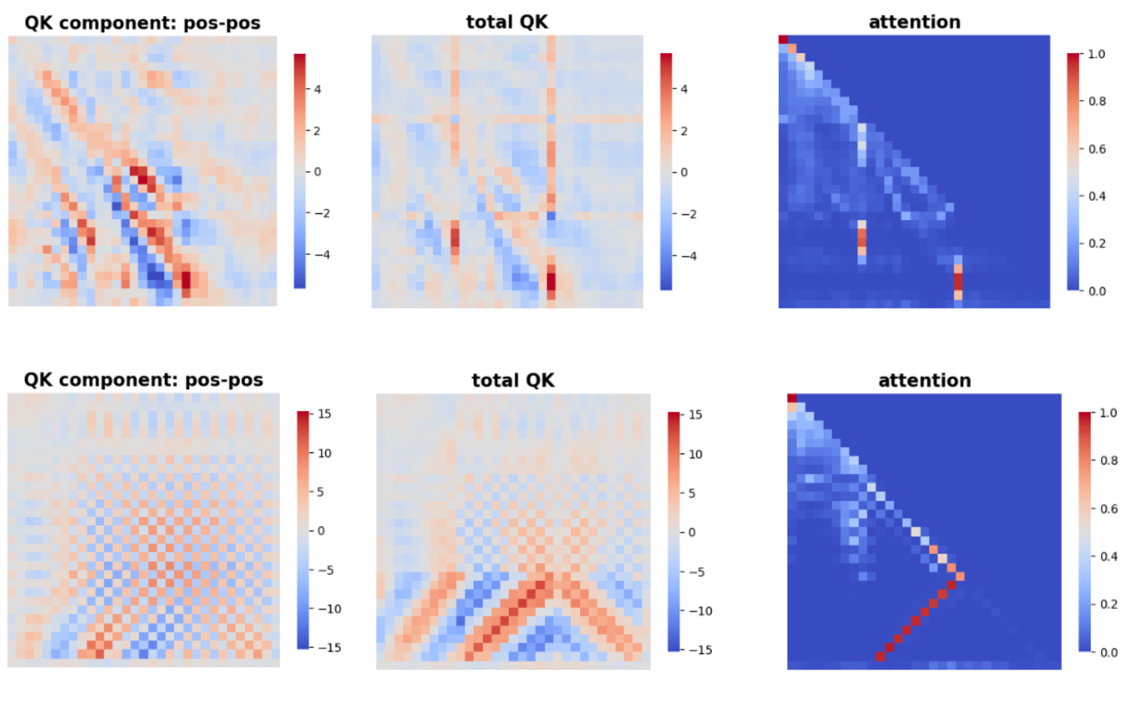
Discontinuity is a visible structure in our transformer trained on addition inputs. If digits are shortened, lengthened, or shifted in the test data, it will be hard for the model to locate the positions correctly! It seems reasonable to

For math-related tasks, instability issues may arise from discontinuity patterns inside a transformer, making generalization and extrapolation fail.

Final thoughts

Many LLMs are being developed and employed in applications every month. No doubt, interpretability-enhanced LLMs would make our society much safer. While lots of things need to be done, recent research does provide hope for more interpretable models. Here are some questions I think are interesting to explore.

1. How does geometry in transformers increase interpretability? Can we devise informative visualization methods and reliable measurements to monitor what is happening inside black-box models?
2. Can we characterize the smoothness of training data more precisely? If we observe discontinuity patterns, how do we overcome the shortcoming of current transformer models?