Imbalance troubles: Why is the minority class hurt more by overfitting?
This post is based on a recent paper.
Prelude: Overfitting in neural networks
Deep neural networks such as ResNets and Transformers are standard recipes for classification. They are powerful feature extractors that learn feature representations of data as vectors in high dimensions. They have a tendancy to fit data well—often achieving 100% train accuracy. In fact, a well-known paper shows that popular CNN models can be easily trained to fit corrupted labels (a fraction of labels are arbitrarily permuted). This paper was a bit shocking because of a deep-rooted belief in statistics: a model can’t memorize and generalize well at the same time (Bias-variance tradeoff).
Since then, a lot of research activities have focused on understanding why neural networks generalize well on test data despite perfect fits. The notion of benign overfitting and subsequent research seem to have largely resolved the puzzle. The key idea is that when the model has a large number of parameters (thus achieving the perfect train accuracy), then there is an implicit regularization effect that encourages the model to be parsimonious. In the simple case of linear classification, when training data is linearly separable, then max-margin classifier is the “preferred” classifier.
Overfitting headache in imbalanced classification

Many datasets are highly imbalanced, which means that there are minority classes whose training samples are much fewer than the other classes (majority classes). Data imbalance is especially common in downstream analysis. For example, doctors want to classify medical images by leveraging existing models; but images with diseases (say cancer) are often scarce.
A common practice is to take a pretrained neural network (for example, ResNets or vision Transformers) and use it as a feature extractor. For each image, we will have a feature vector \(\boldsymbol{x}_i\) using the neural network. If we have labels \(y_i\) (\(i=1,2,\ldots,n\)) for the images on a downstream task, then we can simply train a linear classifier such as logistic regression or support vector machine (SVM) using the dataset \((\boldsymbol{x}_i, y_i)\). (A more sophisticated approach is to finetune the last few layers of the nerual net, but we won’t discuss this here.)
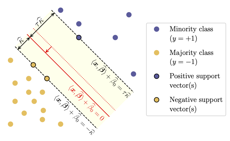
Suppose that we only have two classes (\(y_i \in \{\pm 1\}\)) and the training data is linear separable, namely, there exists a vector \(\boldsymbol{\beta}\) such that \(\boldsymbol{\beta}^\top x_i > 0\) if and only if \(y_i=1\). The implicit bias of gradient descent algorithms is known to promote the max-margin classifier, which can be obtained by including a tiny \(\ell_2\) regularization or running the gradient descent for sufficiently long time. After fitting a max-margin classifier, we obtain the coefficients \((\boldsymbol{\beta}, \beta_0)\) where \(\beta_0\) is the intercept term.

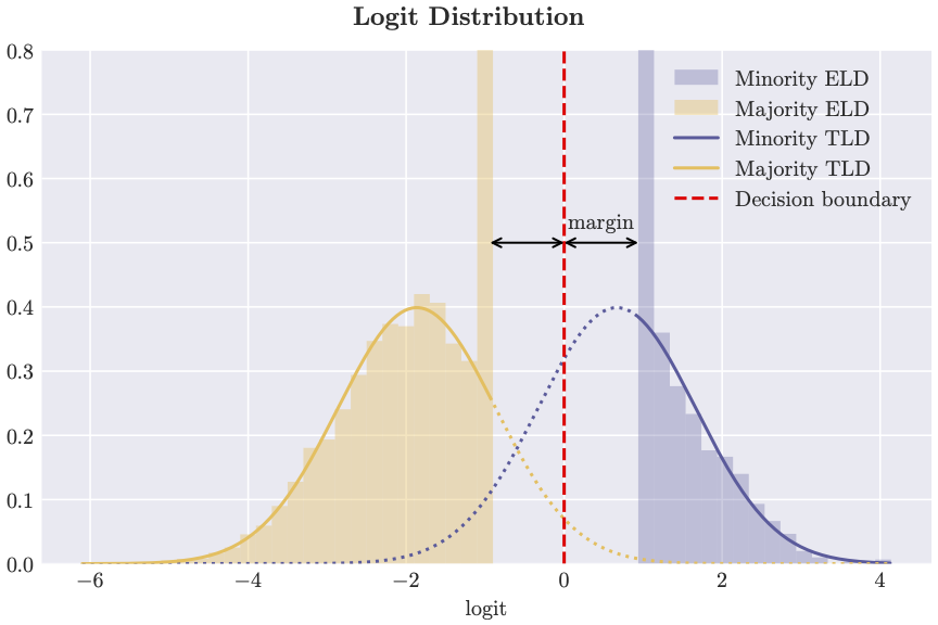
The logit usually refers to the real-valued scalar before we apply Softmax to get prediction probabilities. In our case, for a feature \(\boldsymbol{x}\), the logit is \(\boldsymbol{\beta}^\top \boldsymbol{x} + \beta_0\). In the figure above, we generated features from a mixture of two Gaussians, and fit a max-margin classifier. Then we plotted the distribution of logits on the training dataset as histograms which are fitted by solid curves, and the distribution of logits on the test dataset fitted by dashed curves. Two colors indicate the two classes. We’ve also found similar results across various data modalities, including tabular data, image data, and text data.
What do we discover? The logit distributions are clearly different on train vs. test datasets. More concretely,
- The logit distributions on the training dataset look like truncated Gaussian distributions;
- The minority logit distribution (right cluster, histogram rescaled for better visibility) is “eaten” more by the truncation, thus having worse accuracy.
Hmmm, why is there a bigger discrepancy for the minority class in terms of logit distributions between the training dataset vs. the test dataset? A branch of statistical theory, high-dimensional statistics, offers perfect tools for understanding such phenomenon.
A tour of recent statistical theory: trouble of high dimensionality
In statistics, a classifier obtained from a training dataset is viewed as inherently random, because the training examples are random samples from the universe of all possible examples (known as population); Think about drawing a different training dataset, then the classifier should also be different. But fortunately, for linear classifiers, classical statistical theory tells us that the variability is small if the feature dimension \(d\) is much smaller than the sample size \(n\). For our previous experiment, we would expect small when \(d \ll n\).
- Consistency: \(\boldsymbol{\beta}\) is close to the “true” coefficient vector \(\boldsymbol{\beta}\) if we had infinite training samples.
- Normal distribution: the logit distribution is a projection of multivariate features into 1D, which is univariate Gaussian (recall that linear projection of multivariate Gaussian is still Gaussian).
However, this classical picture falls apart if \(d\) and \(n\) are comparable. When the dimension is getting large, there is too much flexibility (known as degree of freedom) for a classifier to fit the training data, so it gets more “uncertain”. Roughly speaking, this is the source of overfitting when the dimension is too large or the model has a higher fitting capability.
It turns out that there is a phase transition phenomenon: there exists a critical threshold for \(d/n\), above which the training data is linearly separable, and the maximum likelihood estimation (MLE) is not well defined. See this paper for example.
To understand intuitively why dimensionality matters for classification problems, consider a simple case where \(n=d\) and each feature is one of the canonical basis, that is, the \(i\)-th coordinate of \(\boldsymbol{x}_i\) is 1 and other coordinates are 0. Then for any positive scaler \(c\), the coefficient vector \(\sum_{i=1}^n \big[ c \mathbf{1}\{y_i=1\} - \mathbf{1}\{y_i=-1\} \big] \boldsymbol{x}_i\) perfectly separates the two classes, no matter what labels \(y_i\) are. This simple case is actually not that artificial, as \(n\) points in general position in a \(d\)-dimensional space with \(d \ge n\) can be mapped to the canonical basis by an affine transformation.
Rethinking overfitting through logit distribution
All is not lost when we are in very high dimensions. As we saw earlier, the max-margin linear classifier—which is unique and has often generalizes well—is the “preferred” classifier thanks to implicit regularization. But overfitting does create an issue for the minority class.
Our theory finds that the distortion (truncation) of logit distributions completely explains overfitting. The following heuristic explanations are derived from our theory.
- High dimensionality allows arbitrary distortion of logit distributions up to a certain limit (measured by the Wasserstein distance);
- Since the minority class weights less and counts less toward the limit, its logit distribution is more severely distorted in order to maximize the margin;
- Large distortion of the minority logit distribution leads to worse test accuracy, despite perfect train accuracy.
Some of the intuitions (especially the first point) and technical tools already appear in prior work such as this paper on projection pursuit.
Consequence and margin rebalancing
Our analysis reveals that data imbalance not only exacerbates test accuray for the minority class, but increases errors for calibration as well. The general trend we’ve found can be summarized by the following.
In terms of impact on test accuracy and calibration, degree of data imbalance \(\approx\) noise level.
What can we do to counter overfitting for the minority class? In many applications such as medical image classification, we want the minority class to be correctly classified as much as the majority class. We studied a common strategy where margins are rebalanced based on the sample sizes of both classes.

In some situations, we discovered that margins rebalancing is indispensable: the balanced test error is as worse as a random guess without margin rebalancing, but is close to zero with appropriate margin rebalancing.
Epilogue: why it matters
Okay, you might say, it is an interesting phenomenon but how it is relevant to machine learning practice? I don’t have a conclusive answer. Arguably our current analysis of linear classifiers is a bit simpler— but it is potentially connected to a wide range of practice in deep learning (feedback is welcome!).
- Pretraining: margin-aware adjustment in the loss function design
- Fine-tuning: distribution shifts and bias correction
- Interpretability: linear probing of features or network activations
Let me give some concrete examples. In computer vision, researchers have used similar intuitions to rebalance margins in designing loss functions for pretraining. When adapting and interpreting language models, linear probing is widely used to distinguish desired features and harmful features.
It is quite conceivable that linear classifiers are building blocks of existing or future AI systems, as models need to represent concepts as clusters in the feature space. For improving AI safety, we’d better understand how bias is generated from training. Analyzing linear classifiers is probably just a starting point!