STAT 709 · Lecture 12 · Unbiased estimation and UMVUE

These notes support STAT 709 at the University of Wisconsin–Madison. Use them alongside the cited textbooks; corrections and questions are welcome.

Exam scope for this lecture.

Section 4 and its linked Exercises 3, 4 and 6 are for understanding and will not be directly tested in exams. Other high- and mid-priority material remains in examination scope.

High priorityOverview

Conditioning. Conditioning removes variation that carries no information about the parameter.
Completeness. Completeness then makes the remaining unbiased function unique.
Applications. We develop this two-step route to uniformly minimum variance unbiased estimation, work through Normal, Uniform, Poisson and exponential examples, and distinguish optimality within unbiased rules from optimality among all estimators.

This begins Part IV. The part overview connects these lectures and includes a final self-check.

Lecture 11 judged estimators as $n\to\infty$ $n\to\infty$ ; this lecture returns to a fixed $n$ $n$ .

Recap from earlier lecturesFrom Lectures 5–7: conditioning, sufficiency and risk · 1 min

Reminder only: this block introduces no new exam requirements.

Sufficiency. Given a sufficient statistic, the conditional data law has a version independent of the unknown parameter. Used in Section 1.
Factorization and exponential families. Factorization separates a parameter-dependent function of a statistic from a parameter-free factor. Used in Section 2.
Conditional means. The tower rule preserves expectations, and conditional averaging cannot increase mean squared error. Used in Section 1.
Bias and MSE. Unbiasedness is one constraint; squared-error risk also includes variance. Used in Section 1.

Learning goals

Compare the MSE of an estimator with that of its conditional average.
Explain why sufficiency is needed for a parameter-independent averaging rule.
Use completeness and Lehmann–Scheffé to identify a UMVUE.
Work through the Section 4 examples for understanding, respecting their exam exemption.

High priorityIntroduction

In previous lectures, we showed that the bias–variance tradeoff is a general phenomenon in statistics. An optimal estimator may not exist or may depend on a case-by-case analysis. However, if we only consider unbiased estimators, there is a systematic way of finding optimal estimators.

1. Motivations

High priorityMotivations

A well-studied question in estimation theory is the construction of optimal (or near-optimal) estimators. After all, there are many ways to find estimators, but some are better than others. Consider the following simple setting. Suppose that we have data $X_1, X_2, \ldots, X_n \stackrel{\mathrm{i.i.d.}}{\sim} \mathcal{E}(\mu)$ $X_1, X_2, \ldots, X_n \stackrel{\mathrm{i.i.d.}}{\sim} \mathcal{E}(\mu)$ where $\mathcal{E}(\mu)$ $\mathcal{E}(\mu)$ is the exponential distribution with parameter $\mu$ $\mu$ , i.e., the pdf is \[f_{\mu}(x) = \frac{1}{\mu} e^{- x / \mu} \mathbf{1}\{ x \ge 0\}.\] $f_{\mu}(x) = \frac{1}{\mu} e^{- x / \mu} \mathbf{1}\{ x \ge 0\}.$ In order to estimate the unknown parameter $\mu > 0$ $\mu > 0$ (assume $n>2$ $n>2$ ), a natural estimator is the sample mean $\bar X$ $\bar X$ since $\mu = \E[X_i]$ $\mu = \mathbb{E}[X_i]$ . But imagine that a portion of the data—$X_1, X_2$ $X_1, X_2$ —is stored in one data center or server, and the rest is stored in another data center. Each data center may estimate $\mu$ $\mu$ with \[\hat \mu_1 = \frac{1}{2} (X_1 + X_2), \qquad \hat \mu_2 = \frac{1}{n-2} \sum_{i>2} X_i.\] $\hat \mu_1 = \frac{1}{2} (X_1 + X_2), \qquad \hat \mu_2 = \frac{1}{n-2} \sum_{i>2} X_i.$ We can combine the two estimators from the two data centers: \[\hat \mu_3 = \frac{1}{2} (\hat \mu_1 + \hat \mu_2).\] $\hat \mu_3 = \frac{1}{2} (\hat \mu_1 + \hat \mu_2).$ Which one should we choose? The principle of sufficiency says that we should choose an estimator that “sufficiently” summarizes the data. We can check that $\hat\mu_1$ $\hat\mu_1$ and $\hat\mu_2$ $\hat\mu_2$ are not individually sufficient; $\hat\mu_3$ $\hat\mu_3$ is generally not sufficient either (except when $n=4$ $n=4$ , when it equals $\bar X$ $\bar X$ ), but $(\hat \mu_1, \hat \mu_2)$ $(\hat \mu_1, \hat \mu_2)$ is a sufficient statistic.

Conditioning reduces variance.

If $\E Y^2<\infty$ $\mathbb{E}Y^2<\infty$ and $Z$ $Z$ is any random variable, then

\[\mathrm{Var}(\E[Y\mid Z])\le\mathrm{Var}(Y).\] $\mathrm{Var}(\mathbb{E}[Y\mid Z])\le\mathrm{Var}(Y).$

(1)

This follows from the variance decomposition discussed in Section 4.2 of Lecture 5.

Instructor’s NoteConditioning and the unknown parameter

Unbiasedness is unnecessary. Think of conditioning as averaging away some of the estimator’s noise. This averaging keeps the estimator’s mean, and hence its bias, unchanged. Its variance goes down, so its mean squared error goes down too, even if we started with a biased estimator.

Sufficiency makes the averaging rule usable. Write the model parameter as $\theta$ $\theta$ ($\mu$ $\mu$ in the example above). When we form \[\mathbb E_\theta[T_2(X)\mid T_1(X)]=g_\theta(T_1(X)),\] $\mathbb E_\theta[T_2(X)\mid T_1(X)]=g_\theta(T_1(X)),$ the subscript $\theta$ $\theta$ matters: the expectation is taken under the probability measure $P_\theta$ $P_\theta$ , which depends on the unknown parameter. Without sufficiency, conditioning can bring that unknown $\theta$ $\theta$ into the resulting rule. Then $g_\theta(T_1(X))$ $g_\theta(T_1(X))$ is not a statistic we can calculate from the data alone. Sufficiency removes $\theta$ $\theta$ from the conditional law of $X$ $X$ given $T_1(X)$ $T_1(X)$ , so the averaging produces one function $g(T_1(X))$ $g(T_1(X))$ that we can actually use. Intuitively, we can average over the variation left after observing $T_1$ $T_1$ without first knowing the parameter we want to estimate.

Why the MSE also decreases.

Fix a model distribution $P_\mu$ $P_\mu$ , suppose $\E_\mu[T_2(X)^2]<\infty$ $\mathbb{E}_\mu[T_2(X)^2]<\infty$ , and set $g_\mu(T_1)=\E_\mu[T_2(X)\mid T_1(X)]$ $g_\mu(T_1)=\mathbb{E}_\mu[T_2(X)\mid T_1(X)]$ . For any statistic $T_1$ $T_1$ , the exact identity is

\[\E_\mu[(T_2-\mu)^2] =\E_\mu[(g_\mu(T_1)-\mu)^2] +\E_\mu[\Var_\mu(T_2\mid T_1)].\] $\mathbb{E}_\mu[(T_2-\mu)^2] =\mathbb{E}_\mu[(g_\mu(T_1)-\mu)^2] +\mathbb{E}_\mu[\mathrm{Var}_\mu(T_2\mid T_1)].$

(2)

Consequently, $\E_\mu[(g_\mu(T_1)-\mu)^2]\le\E_\mu[(T_2-\mu)^2]$ $\mathbb{E}_\mu[(g_\mu(T_1)-\mu)^2]\le\mathbb{E}_\mu[(T_2-\mu)^2]$ . Unbiasedness is not required. The tower rule gives $\E_\mu g_\mu(T_1)=\E_\mu T_2$ $\mathbb{E}_\mu g_\mu(T_1)=\mathbb{E}_\mu T_2$ , so conditioning preserves the bias while reducing variance. If $T_2$ $T_2$ is unbiased, the conditional version is unbiased too. The reduction is strict at a given $\mu$ $\mu$ exactly when $\E_\mu\Var_\mu(T_2\mid T_1)>0$ $\mathbb{E}_\mu\mathrm{Var}_\mu(T_2\mid T_1)>0$ ; equality holds exactly when $T_2=g_\mu(T_1)$ $T_2=g_\mu(T_1)$ almost surely under $P_\mu$ $P_\mu$ . See Exercise 7 for the complete decomposition proof.

What sufficiency contributes.

Role of sufficiency. Sufficiency is not needed for the inequality at a fixed model distribution. Its role is to make the conditional expectation a usable estimator: a sufficient $T_1$ $T_1$ allows one common function $g$ $g$ , independent of the unknown $\mu$ $\mu$ , with $g(T_1)=\E_\mu[T_2\mid T_1]$ $g(T_1)=\mathbb{E}_\mu[T_2\mid T_1]$ for every $\mu$ $\mu$ . Without sufficiency, the function $g_\mu$ $g_\mu$ may depend on the parameter we are trying to estimate.
Why the distinction matters. For example, if $X\sim\mathcal E(\mu)$ $X\sim\mathcal E(\mu)$ , $T_2=X$ $T_2=X$ and $T_1\equiv0$ $T_1\equiv0$ , then $g_\mu(T_1)=\mu$ $g_\mu(T_1)=\mu$ . Its MSE is zero, but we cannot compute it from the data without already knowing $\mu$ $\mu$ .
General guarantee. A nonsufficient statistic can still work for a particular $T_2$ $T_2$ ; sufficiency supplies the general guarantee. This is the Rao–Blackwell theorem, which does not require completeness. See Theorem 2.5 of [1] and Shao’s Stat 609 notes, slides 13–15.

Since there are many ways to find sufficient statistics, it is natural to seek a sufficient statistic that is minimal in a certain sense; in the motivating example, both $(\hat \mu_1, \hat \mu_2)$ $(\hat \mu_1, \hat \mu_2)$ and $\bar X$ $\bar X$ are sufficient statistics, but $\bar X$ $\bar X$ is simpler because it is a function of $(\hat \mu_1, \hat \mu_2)$ $(\hat \mu_1, \hat \mu_2)$ . Completeness is a separate property: it will ensure uniqueness of unbiased functions of a sufficient statistic.

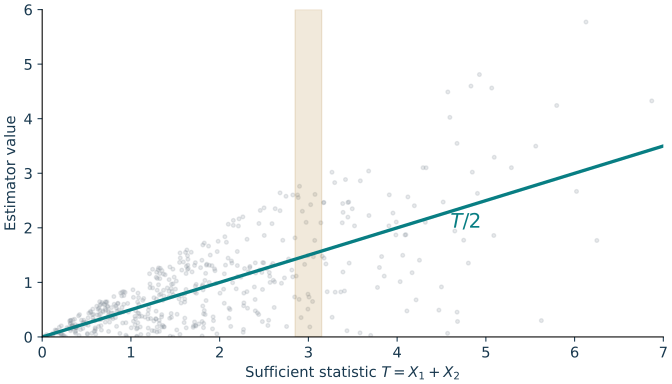
For two independent Exponential observations of mean one in this illustration, points show X1 versus the sufficient sum T. Conditional averaging gives T/2, preserving the mean and halving the variance.

As a separate illustration, let $X_1,X_2$ $X_1,X_2$ be independent exponential observations with unknown mean $\theta$ $\theta$ . Their sum $T$ $T$ is sufficient, and symmetry gives $\E_\theta[X_1\mid T]=T/2$ $\mathbb{E}_\theta[X_1\mid T]=T/2$ . Both estimate $\theta$ $\theta$ without bias, but their variances are $\theta^2$ $\theta^2$ and $\theta^2/2$ $\theta^2/2$ . The synthetic scatter uses $\theta=1$ $\theta=1$ and 500 pairs; it illustrates within-group variation rather than proving the identity.

Conditioning and variance.

For square-integrable $Y$ $Y$ , $\Var(Y)=\Var(\E[Y\mid T])+\E\Var(Y\mid T)$ $\mathrm{Var}(Y)=\mathrm{Var}(\mathbb{E}[Y\mid T])+\mathbb{E}\mathrm{Var}(Y\mid T)$ . Conditioning removes the second nonnegative term while preserving the mean.

Mid priorityPractice: Weighting two independent server means

See Exercise 1 in Section 7 for the full statement and complete solution.

2. Complete statistics

Mid priorityComplete statistics

Quick Explanation

Minimal sufficiency

Recall that a statistic $T(X)$ $T(X)$ based on data $X = (X_1,\ldots,X_n)$ $X = (X_1,\ldots,X_n)$ drawn from $P \in \mathcal{P}$ $P \in \mathcal{P}$ is sufficient iff it retains relevant information for inferring the unknown distribution $P$ $P$ , or in other words the conditional distribution $X|T(X)$ $X|T(X)$ does not depend on the choice of $P$ $P$ . However, there may be redundant information in $T(X)$ $T(X)$ ; e.g., $T(X) = X$ $T(X) = X$ is trivially sufficient but not practically useful.

We introduce completeness as a criterion for good summary statistics¹.

Definition 1Complete Statistics

$T(X)$ $T(X)$ is complete for the family $\mathcal{P}$ $\mathcal{P}$ if and only if for all Borel functions $f$ $f$ with $\E_P|f(T)|<\infty$ $\mathbb{E}_P|f(T)|<\infty$ for every $P\in\mathcal P$ $P\in\mathcal P$ , $\mathbb{E}_P[f(T)] = 0$ $\mathbb{E}_P[f(T)] = 0$ , $\forall P \in \mathcal{P}$ $\forall P \in \mathcal{P}$ implies that $f(T) = 0$ $f(T) = 0$ a.s. $P$ $P$ .

From this definition, if $T(X)$ $T(X)$ is complete and $\psi$ $\psi$ , $\psi^{-1}$ $\psi^{-1}$ are one-one measurable functions, then $\psi(T(X))$ $\psi(T(X))$ is also complete. It is easy to find complete statistics in an exponential family.

Proposition 1

Let $\mathcal{P} = \{P_\eta: \eta \in \Xi\}$ $\mathcal{P} = \{P_\eta: \eta \in \Xi\}$ be an exponential family of full rank (contains an open set) with p.d.f. given by \[f_\eta(x) = \exp\{\eta^{\text{T}}T(x) - \xi(\eta)\}h(x).\] $f_\eta(x) = \exp\{\eta^{\text{T}}T(x) - \xi(\eta)\}h(x).$ Then $T(X)$ $T(X)$ is sufficient and complete for $\eta \in \Xi$ $\eta \in \Xi$ .

Below are examples taken from [1] (Examples 2.15–2.17).

Example 1

Let $X_1, \ldots, X_n \stackrel{\iid}{\sim} \mathcal{N}(\mu, \sigma^2)$ $X_1, \ldots, X_n \stackrel{\mathrm{i.i.d.}}{\sim} \mathcal{N}(\mu, \sigma^2)$ , $\mu \in \mathbb{R}$ $\mu \in \mathbb{R}$ , $\sigma^2 > 0$ $\sigma^2 > 0$ . The joint p.d.f. of $X_1, \ldots, X_n$ $X_1, \ldots, X_n$ is \[(2\pi)^{-n/2}\exp\{\eta_1T_1 + \eta_2 T_2 - n \xi(\eta)\},\] $(2\pi)^{-n/2}\exp\{\eta_1T_1 + \eta_2 T_2 - n \xi(\eta)\},$ where $T_1 = \sum_{i=1}^{n} X_i$ $T_1 = \sum_{i=1}^{n} X_i$ , $T_2 = -\sum_{i=1}^{n} X_i^2$ $T_2 = -\sum_{i=1}^{n} X_i^2$ , and $\eta = (\eta_1, \eta_2) = (\frac{\mu}{\sigma^2}, \frac{1}{2\sigma^2})$ $\eta = (\eta_1, \eta_2) = (\frac{\mu}{\sigma^2}, \frac{1}{2\sigma^2})$ . Thus, $T = (T_1, T_2)$ $T = (T_1, T_2)$ is complete and sufficient for $\eta$ $\eta$ . Also, $(\bar{X}, S^2)$ $(\bar{X}, S^2)$ is complete and sufficient for $\theta=(\mu,\sigma^{2})$ $\theta=(\mu,\sigma^{2})$ .

Example 2

Let $X_1, \ldots, X_n \stackrel{i.i.d.}{\sim} P_\theta = U(0, \theta)$ $X_1, \ldots, X_n \stackrel{i.i.d.}{\sim} P_\theta = U(0, \theta)$ , $\theta > 0$ $\theta > 0$ . Check that $X_{(n)}$ $X_{(n)}$ is complete and sufficient for $\theta>0$ $\theta>0$ .

Example 3

Let $\mathcal{P}$ $\mathcal{P}$ be the family of all distributions on $\mathbb{R}$ $\mathbb{R}$ having a Lebesgue p.d.f., and let the sample be i.i.d. Then $T(X) = (X_{(1)}, \ldots, X_{(n)})$ $T(X) = (X_{(1)}, \ldots, X_{(n)})$ is complete for $\mathcal{P}$ $\mathcal{P}$ .

Proof. Let $\mathcal{P}_0$ $\mathcal{P}_0$ be exponential family \[f(x) = C(\theta_1, \ldots, \theta_n) \exp(-x^{2n} + \theta_1 x + \theta_2 x^2 + \cdots + \theta_n x^n),\] $f(x) = C(\theta_1, \ldots, \theta_n) \exp(-x^{2n} + \theta_1 x + \theta_2 x^2 + \cdots + \theta_n x^n),$ where $C(\theta_1, \cdots, \theta_n)$ $C(\theta_1, \cdots, \theta_n)$ is the normalizing constant. $\mathcal{P}_0 \subset \mathcal{P}$ $\mathcal{P}_0 \subset \mathcal{P}$ , and $(\sum X_i, \ldots, \sum X_i^n)$ $(\sum X_i, \ldots, \sum X_i^n)$ is complete for $\mathcal{P}_{0}$ $\mathcal{P}_{0}$ . Since every density in $\mathcal P_0$ $\mathcal P_0$ is strictly positive on $\R$ $\mathbb{R}$ , a null event for its i.i.d. sample law is Lebesgue-null on $\R^n$ $\mathbb{R}^n$ and hence null for every i.i.d. sample law with a Lebesgue density, $(\sum X_i, \ldots, \sum X_i^n)$ $(\sum X_i, \ldots, \sum X_i^n)$ is complete for $\mathcal{P}$ $\mathcal{P}$ . There exists one-one mapping $(\sum X_i, \ldots, \sum X_i^n) \leftrightarrow (X_{(1)}, \ldots, X_{(n)})$ $(\sum X_i, \ldots, \sum X_i^n) \leftrightarrow (X_{(1)}, \ldots, X_{(n)})$ . Therefore, $(X_{(1)}, \ldots, X_{(n)})$ $(X_{(1)}, \ldots, X_{(n)})$ is complete for $\mathcal P$ $\mathcal P$ . ◻

Instructor’s NoteNo invisible unbiased correction

Intuition. Completeness says that a function of the summary cannot secretly add a nonzero correction whose average is zero under every possible parameter.
Interpretation. Once a complete sufficient summary has produced an unbiased answer, there is no second unbiased answer hidden inside that same summary.

Mid priorityPractice: Completeness for one Bernoulli variable

See Exercise 2 in Section 7 for the full statement and complete solution.

3. UMVUE

High priorityUMVUE

Quick Recall

Conditioning and variance

Recall that we say $T(X)$ $T(X)$ is unbiased for an unknown parameter $\nu$ $\nu$ if and only if \[\begin{aligned} \mathbb{E}[T(X)] = \nu,\quad \forall P \in \mathcal{P}. \end{aligned}\] $\begin{aligned} \mathbb{E}[T(X)] = \nu,\quad \forall P \in \mathcal{P}. \end{aligned}$

Definition 2UMVUE

Suppose that $T(X)$ $T(X)$ is unbiased for $\nu(P)$ $\nu(P)$ for every $P\in\mathcal P$ $P\in\mathcal P$ and has a finite second moment under every such $P$ $P$ . We say $T(X)$ $T(X)$ is a uniformly minimum variance unbiased estimator (UMVUE) of $\nu$ $\nu$ if and only if \[\begin{aligned} \mathrm{Var}(T(X)) \le \mathrm{Var}(U(X)),\quad\forall P \in \mathcal{P},\quad \forall \text{ unbiased } U(X). \end{aligned}\] $\begin{aligned} \mathrm{Var}(T(X)) \le \mathrm{Var}(U(X)),\quad\forall P \in \mathcal{P},\quad \forall \text{ unbiased } U(X). \end{aligned}$

It is clear that UMVUE implies optimality among all unbiased estimators in terms of mean squared error (MSE). For general loss functions instead of the quadratic loss, “minimum variance” is replaced by “minimum risk.”

Remark 1

UMVUE does not always exist a priori. For fixed $P \in \mathcal{P}$ $P \in \mathcal{P}$ , we can solve \[\begin{aligned} \min_{\text{unbiased }T} \mathrm{Var}(T(X)), \end{aligned}\] $\begin{aligned} \min_{\text{unbiased }T} \mathrm{Var}(T(X)), \end{aligned}$ but the minimizer is not guaranteed to be uniform for every $P \in \mathcal{P}$ $P \in \mathcal{P}$ .

The following Lehmann–Scheffé theorem [1][Thm. 3.1] states that given a sufficient and complete statistic, often we can find a UMVUE.

Theorem 1Lehmann–Scheffé

Suppose that there exists a sufficient and complete statistic $T(X)$ $T(X)$ for $\mathcal{P}$ $\mathcal{P}$ . If $\nu$ $\nu$ admits an unbiased estimator with finite second moment under every $P\in\mathcal P$ $P\in\mathcal P$ , then there exists a unique² UMVUE, which is of the form $h(T)$ $h(T)$ where $h$ $h$ is a Borel function.

Proof. This is a consequence of the Rao–Blackwell Theorem and completeness, which we prove below. If $U(X)$ $U(X)$ is unbiased for $\nu$ $\nu$ , then by (1), \[\begin{aligned} \mathrm{Var}(\mathbb{E}[U|T]) \le \mathrm{Var}(U). \end{aligned}\] $\begin{aligned} \mathrm{Var}(\mathbb{E}[U|T]) \le \mathrm{Var}(U). \end{aligned}$ Note that $\mathbb{E}[U|T]$ $\mathbb{E}[U|T]$ is a function of $T$ $T$ , i.e. $\mathbb{E}[U|T] = h(T)$ $\mathbb{E}[U|T] = h(T)$ . Sufficiency permits a version of $h$ $h$ that does not depend on the unknown parameter. For two unbiased starting estimators, their two conditional functions have difference with mean zero for every $P$ $P$ ; completeness makes that difference zero almost surely. Thus $h(T)$ $h(T)$ does not depend on the choice of $U$ $U$ , up to these null sets, so $h(T)$ $h(T)$ has minimum variance among all unbiased estimators $U$ $U$ , which implies that $h(T)$ $h(T)$ is UMVUE.

If $\tilde{T}$ $\tilde{T}$ is another UMVUE, then the variance of $\mathbb{E}[\tilde{T}|T]$ $\mathbb{E}[\tilde{T}|T]$ must be no larger than that of $h(T)$ $h(T)$ , thus equal. Since MSE is based on a strictly convex loss, $\tilde{T}$ $\tilde{T}$ must be a function of $T$ $T$ (by [1] (Theorem 2.5)). Therefore, $\tilde{T} = h(T)$ $\tilde{T} = h(T)$ a.s. $\forall P \in \mathcal{P}$ $\forall P \in \mathcal{P}$ . ◻

The UMVUE route.

Sufficiency makes Rao–Blackwell conditioning independent of the unknown parameter. Completeness then makes unbiased functions of that statistic unique, giving the Lehmann–Scheffe route to a UMVUE.

4. Three ways to find UMVUE

Mid priorityThree ways to find UMVUE

How to study this section.

It is good to go through the examples and proofs at least once to understand how the methods work. This section will not be directly tested in exams. The mid-priority blocks guide your study; Method 3 remains low priority.

We will introduce three ways of finding UMVUEs. Examples are taken from [1][Section 3.1].

4.1. Method 1

Mid priorityMethod 1

Quick Recall

Completeness

Find sufficient and complete statistic $T(X)$ $T(X)$ , then find $h(T)$ $h(T)$ , such that \[\begin{aligned} \mathbb{E}[h(T)] = \nu,\quad \forall P \in \mathcal{P}. \end{aligned}\] $\begin{aligned} \mathbb{E}[h(T)] = \nu,\quad \forall P \in \mathcal{P}. \end{aligned}$

Example 4Example 3.1

Let $X_1, \ldots, X_n \stackrel{\iid}{\sim}\text{Unif}([0, \theta])$ $X_1, \ldots, X_n \stackrel{\mathrm{i.i.d.}}{\sim}\text{Unif}([0, \theta])$ , $\theta > 0$ $\theta > 0$ . Let $\nu = g(\theta)$ $\nu = g(\theta)$ with $g\in C^1((0,\infty))$ $g\in C^1((0,\infty))$ . We know that $X_{(n)} = \max_{1\le i \le n} X_i$ $X_{(n)} = \max_{1\le i \le n} X_i$ is complete, with p.d.f. given by \[\begin{aligned} f_{\theta}(x) = n\frac{1}{\theta^n}x^{n-1}I_{(0, \theta)}(x). \end{aligned}\] $\begin{aligned} f_{\theta}(x) = n\frac{1}{\theta^n}x^{n-1}I_{(0, \theta)}(x). \end{aligned}$ Our goal is to find $h$ $h$ , such that \[\begin{aligned} \theta^n g(\theta) = n\int_{0}^{\theta}h(x)x^{n-1}dx. \end{aligned}\] $\begin{aligned} \theta^n g(\theta) = n\int_{0}^{\theta}h(x)x^{n-1}dx. \end{aligned}$ Taking the derivative on both sides, we get \[\begin{aligned} n\theta^{n-1}g(\theta) + \theta^n g'(\theta) = nh(\theta)\theta^{n-1}. \end{aligned}\] $\begin{aligned} n\theta^{n-1}g(\theta) + \theta^n g'(\theta) = nh(\theta)\theta^{n-1}. \end{aligned}$ Rearranging gives $h(x)=g(x)+xg'(x)/n$ $h(x)=g(x)+xg'(x)/n$ . For unbiasedness, also require $\lim_{x\downarrow0}x^ng(x)=0$ $\lim_{x\downarrow0}x^ng(x)=0$ and integrability of $h(x)x^{n-1}$ $h(x)x^{n-1}$ on $(0,\theta)$ $(0,\theta)$ ; for UMVUE require its square integrability. The boundary term is essential: differentiating the integral equation alone can lose a nonzero integration constant. In particular, if $\nu = \theta$ $\nu = \theta$ , then \[\begin{aligned} h(X_{(n)}) = (1+\frac{1}{n})X_{(n)}. \end{aligned}\] $\begin{aligned} h(X_{(n)}) = (1+\frac{1}{n})X_{(n)}. \end{aligned}$

Example 5Example 3.2

Let $X_1,\ldots,X_n\stackrel{\iid}{\sim}\mathrm{Poisson}(\theta)$ $X_1,\ldots,X_n\stackrel{\mathrm{i.i.d.}}{\sim}\mathrm{Poisson}(\theta)$ , $\theta>0$ $\theta>0$ . The total $S=\sum X_i\sim\mathrm{Poisson}(n\theta)$ $S=\sum X_i\sim\mathrm{Poisson}(n\theta)$ is complete sufficient because its natural parameter ranges over $\R$ $\mathbb{R}$ . The identities $\E S=n\theta$ $\mathbb{E}S=n\theta$ and $\E S(S-1)=n^2\theta^2$ $\mathbb{E}S(S-1)=n^2\theta^2$ show that $S/n$ $S/n$ and $S(S-1)/n^2$ $S(S-1)/n^2$ are UMVUEs of $\theta$ $\theta$ and $\theta^2$ $\theta^2$ , respectively.

Example 6Example 3.6

Let $X_1, \ldots, X_n \stackrel{i.i.d.}{\sim} P \in \mathcal{P}$ $X_1, \ldots, X_n \stackrel{i.i.d.}{\sim} P \in \mathcal{P}$ , where $\mathcal{P}$ $\mathcal{P}$ is the family of all distributions with a Lebesgue p.d.f. satisfying the moment conditions specified below, and $n\ge2$ $n\ge2$ . Let $T = (X_{(1)}, \ldots, X_{(n)})$ $T = (X_{(1)}, \ldots, X_{(n)})$ be a complete and sufficient statistic. Note that $\varphi(X_1, \ldots, X_n)$ $\varphi(X_1, \ldots, X_n)$ is a function of $T$ $T$ if and only if for any permutation $\pi$ $\pi$ , \[\begin{aligned} \varphi(X_1, \ldots, X_n) = \varphi(X_{\pi(1)}, \ldots, X_{\pi(n)}). \end{aligned}\] $\begin{aligned} \varphi(X_1, \ldots, X_n) = \varphi(X_{\pi(1)}, \ldots, X_{\pi(n)}). \end{aligned}$ We use $T$ $T$ to construct UMVUEs on the relevant moment classes: finite second moment for the mean and squared mean, and finite fourth moment for the variance rule. These assumptions ensure finite estimator variance. Writing $S^2=(n-1)^{-1}\sum_i(X_i-\bar X)^2$ $S^2=(n-1)^{-1}\sum_i(X_i-\bar X)^2$ , the squared-mean rule has the cancellation \[\frac1n\sum_iX_i^2-S^2 =\frac{2}{n(n-1)}\sum_{i<j}X_iX_j.\] $\frac1n\sum_iX_i^2-S^2 =\frac{2}{n(n-1)}\sum_{i<j}X_iX_j.$ Each product has finite second moment because independence gives $\E(X_iX_j)^2=(\E X_1^2)^2<\infty$ $\mathbb{E}(X_iX_j)^2=(\mathbb{E}X_1^2)^2<\infty$ . Thus a fourth moment is unnecessary for this rule, although it is sufficient for the variance estimator $S^2$ $S^2$ .

(1) $\nu = \mathbb{E}[X_i]$ $\nu = \mathbb{E}[X_i]$ . Then $\bar{X}$ $\bar{X}$ .
(2) $\nu = \mathrm{Var}(X_i)$ $\nu = \mathrm{Var}(X_i)$ . Then $S^2$ $S^2$ .
(3) $\nu = (\mathbb{E}[X_i])^2$ $\nu = (\mathbb{E}[X_i])^2$ . Then $\frac{1}{n}\sum_{i=1}^{n}X_i^2 - S^2$ $\frac{1}{n}\sum_{i=1}^{n}X_i^2 - S^2$ . Note that generally $\mathbb{E}[\bar{X}^2] > (\mathbb{E}[\bar{X}])^2 = (\mathbb{E}[X_i])^2$ $\mathbb{E}[\bar{X}^2] > (\mathbb{E}[\bar{X}])^2 = (\mathbb{E}[X_i])^2$ .
(4) $\nu = \mathbb{P}(X_i \le t)$ $\nu = \mathbb{P}(X_i \le t)$ . Then $F_n(t) = \frac{1}{n} \sum_{i=1}^{n}I_{(-\infty, t]}(X_i)$ $F_n(t) = \frac{1}{n} \sum_{i=1}^{n}I_{(-\infty, t]}(X_i)$ .

Mid priorityPractice: Estimating a Poisson zero probability

See Exercise 3 in Section 7 for the full statement and complete solution.

4.2. Method 2

Mid priorityMethod 2

Find a sufficient and complete $T(X)$ $T(X)$ and an unbiased $U(X)$ $U(X)$ , then apply conditioning (as in the proof at Sec 3). Note that any unbiased $U(X)$ $U(X)$ (as long as its second moment exists) is okay. We have the freedom to choose one so that $\mathbb{E}[U|T]$ $\mathbb{E}[U|T]$ is easy to simplify.

Example 7Binomial

Let $X_1, \ldots, X_n \stackrel{\iid}{\sim}\text{Bin}(k, \theta)$ $X_1, \ldots, X_n \stackrel{\mathrm{i.i.d.}}{\sim}\text{Bin}(k, \theta)$ , where $k$ $k$ is known, $\theta \in (0, 1)$ $\theta \in (0, 1)$ is unknown. Need to calculate \[\begin{aligned} \mathbb{E}[I(X_i=1)|T] = \mathbb{P}(X_i=1|T), \end{aligned}\] $\begin{aligned} \mathbb{E}[I(X_i=1)|T] = \mathbb{P}(X_i=1|T), \end{aligned}$ where $T = \sum_{i=1}^{n}X_i$ $T = \sum_{i=1}^{n}X_i$ . For $S=T=s$ $S=T=s$ , the $nk$ $nk$ Bernoulli trials have $s$ $s$ successes uniformly placed among their positions. Therefore \[\PR(X_1=1\mid S=s)=\frac{\binom{k}{1}\binom{(n-1)k}{s-1}}{\binom{nk}{s}},\qquad 0\le s\le nk,\] $\mathbb{P}(X_1=1\mid S=s)=\frac{\binom{k}{1}\binom{(n-1)k}{s-1}}{\binom{nk}{s}},\qquad 0\le s\le nk,$ with impossible binomial coefficients interpreted as zero. This is the UMVUE of $k\theta(1-\theta)^{k-1}$ $k\theta(1-\theta)^{k-1}$ .

Example 8

(Shao, [1] (Example 3.3)) Let $X_1,\ldots,X_n\stackrel{\iid}{\sim} \mathcal E(\theta)$ $X_1,\ldots,X_n\stackrel{\mathrm{i.i.d.}}{\sim} \mathcal E(\theta)$ with $n\ge2$ $n\ge2$ and take $t\ge0$ $t\ge0$ . We know that \[\begin{aligned} F_\theta(x) = (1-e^{-x/\theta})I_{(0, \infty)}(x). \end{aligned}\] $\begin{aligned} F_\theta(x) = (1-e^{-x/\theta})I_{(0, \infty)}(x). \end{aligned}$ Let $\nu = 1 - F_\theta(t)$ $\nu = 1 - F_\theta(t)$ , then \[\begin{aligned} T(X) = \mathbb{P}(X_1 > t|\bar{X}), \end{aligned}\] $\begin{aligned} T(X) = \mathbb{P}(X_1 > t|\bar{X}), \end{aligned}$ is UMVUE. Note that $\bar{X}$ $\bar{X}$ is complete, and moreover, $\frac{X_1}{\bar{X}}$ $\frac{X_1}{\bar{X}}$ is ancillary since $\mathcal E(\theta)$ $\mathcal E(\theta)$ only has a scale parameter. By Basu’s Theorem (see Theorem 3), $\bar{X}$ $\bar{X}$ is independent of $\frac{X_1}{\bar{X}}$ $\frac{X_1}{\bar{X}}$ . So, \[\begin{aligned} \mathbb{P}(X_1 > t | \bar{X} = \bar{x}) = \mathbb{P}\Big(\frac{X_1}{\bar{X}} > \frac{t}{\bar{X}} | \bar{X} = \bar{x}\Big) = \mathbb{P}\Big(\frac{X_1}{\bar{X}} > \frac{t}{\bar{x}}\Big). \end{aligned}\] $\begin{aligned} \mathbb{P}(X_1 > t | \bar{X} = \bar{x}) = \mathbb{P}\Big(\frac{X_1}{\bar{X}} > \frac{t}{\bar{X}} | \bar{X} = \bar{x}\Big) = \mathbb{P}\Big(\frac{X_1}{\bar{X}} > \frac{t}{\bar{x}}\Big). \end{aligned}$ It remains to derive the p.d.f. of \[\begin{aligned} \frac{X_1}{X_1 + \sum_{i > 1}X_i}. \end{aligned}\] $\begin{aligned} \frac{X_1}{X_1 + \sum_{i > 1}X_i}. \end{aligned}$ Note that $X_1$ $X_1$ is independent of $\sum_{i>1}X_i$ $\sum_{i>1}X_i$ , and $\sum_{i>1}X_i$ $\sum_{i>1}X_i$ has a Gamma distribution. We can use the change-of-variables formula for densities in Lecture 3 to calculate the explicit p.d.f. of this transformation (see Exercise 6). Writing $S=n\bar X$ $S=n\bar X$ , the calculation gives $X_1/S\sim\mathrm{Beta}(1,n-1)$ $X_1/S\sim\mathrm{Beta}(1,n-1)$ independent of $S$ $S$ , and the UMVUE is $(1-t/S)_+^{n-1}$ $(1-t/S)_+^{n-1}$ . This direct calculation supplies the full route without needing the optional Basu theorem.

Example 9Nonexistence of UMVUE

With one observation $X\sim\mathrm{Bernoulli}(p)$ $X\sim\mathrm{Bernoulli}(p)$ , every estimator has expectation $a(1-p)+bp$ $a(1-p)+bp$ , an affine function of $p$ $p$ . It cannot equal $p^2$ $p^2$ for all $p\in(0,1)$ $p\in(0,1)$ . Thus $p^2$ $p^2$ has no unbiased estimator, and consequently no UMVUE, in this experiment.

Remark 2

Let $\mathcal{U}$ $\mathcal{U}$ be the set of all unbiased estimators, \[\begin{aligned} \mathrm{Var}(T(X)) \le \mathrm{Var}(U(X)),~\forall P \in \mathcal{P},~\forall U \in \mathcal{U}. \end{aligned}\] $\begin{aligned} \mathrm{Var}(T(X)) \le \mathrm{Var}(U(X)),~\forall P \in \mathcal{P},~\forall U \in \mathcal{U}. \end{aligned}$ If $\mathcal{P}$ $\mathcal{P}$ is small, $\mathcal{U}$ $\mathcal{U}$ may be large; and conversely, if $\mathcal{P}$ $\mathcal{P}$ is large, then $\mathcal{U}$ $\mathcal{U}$ may be small. A larger parameter space does not imply it is harder to find a UMVUE.

Mid priorityPractice: An unbiased rule for Bernoulli variance

See Exercise 4 in Section 7 for the full statement and complete solution.

4.3. Method 3

Low priority — not examined: Method 3

Find UMVUE without knowing the complete statistics.

Theorem 2Theorem 3.2 of

Let \[\begin{aligned} \mathcal{U} = \{U: \mathbb{E}[U(X)] = 0,~\mathrm{Var}(U(X)) < \infty,~\forall P \in \mathcal{P}\}. \end{aligned}\] $\begin{aligned} \mathcal{U} = \{U: \mathbb{E}[U(X)] = 0,~\mathrm{Var}(U(X)) < \infty,~\forall P \in \mathcal{P}\}. \end{aligned}$ $T$ $T$ is unbiased for $\nu$ $\nu$ with $\mathbb{E}[T(X)^2] < \infty$ $\mathbb{E}[T(X)^2] < \infty$ .

(1) $T(X)$ $T(X)$ is UMVUE if and only if \[\begin{aligned} \mathbb{E}[T(X)U(X)] = 0,~\forall U \in \mathcal{U},~\forall P \in \mathcal{P}. \end{aligned}\] $\begin{aligned} \mathbb{E}[T(X)U(X)] = 0,~\forall U \in \mathcal{U},~\forall P \in \mathcal{P}. \end{aligned}$
(2) If $\tilde{T}$ $\tilde{T}$ is sufficient for $\mathcal{P}$ $\mathcal{P}$ , let \[\begin{aligned} \tilde{\mathcal{U}} = \mathcal{U} \cap \{g(\tilde{T}): g \text{ Borel}\}. \end{aligned}\] $\begin{aligned} \tilde{\mathcal{U}} = \mathcal{U} \cap \{g(\tilde{T}): g \text{ Borel}\}. \end{aligned}$ Then, $T = h(\tilde{T})$ $T = h(\tilde{T})$ is UMVUE if and only if \[\begin{aligned} \mathbb{E}[T(X)U(X)] = 0,~\forall U \in \tilde{\mathcal{U}},~\forall P \in \mathcal{P}. \end{aligned}\] $\begin{aligned} \mathbb{E}[T(X)U(X)] = 0,~\forall U \in \tilde{\mathcal{U}},~\forall P \in \mathcal{P}. \end{aligned}$

Proof. For any zero-mean $U$ $U$ in the stated class, $T+aU$ $T+aU$ is unbiased for every real $a$ $a$ . At fixed $P$ $P$ , \[\Var_P(T+aU)=\Var_P(T)+2a\E_P(TU)+a^2\Var_P(U).\] $\mathrm{Var}_P(T+aU)=\mathrm{Var}_P(T)+2a\mathbb{E}_P(TU)+a^2\mathrm{Var}_P(U).$ If $T$ $T$ is UMVUE, the derivative at $a=0$ $a=0$ must vanish, giving $\E_P(TU)=0$ $\mathbb{E}_P(TU)=0$ . Conversely, any unbiased competitor $V$ $V$ can be written $T+U$ $T+U$ with $\E_PU=0$ $\mathbb{E}_PU=0$ for all $P$ $P$ , so orthogonality gives $\Var_P(V)=\Var_P(T)+\Var_P(U)\ge\Var_P(T)$ $\mathrm{Var}_P(V)=\mathrm{Var}_P(T)+\mathrm{Var}_P(U)\ge\mathrm{Var}_P(T)$ . For (2), first Rao–Blackwellize any competitor on the sufficient statistic and apply the same argument within its functions. ◻

Instructor’s NoteVariation along an unbiased direction

The original calculus-of-variations picture is useful: move a little in any direction that keeps the estimator unbiased. At a minimum, neither sign of that movement can improve the variance, so the linear term must vanish. Here the feasible class is affine; an arbitrary constrained optimization problem need not have zero directional derivatives in every direction.

As a consequence, UMVUE satisfies linearity; see [1][Corollary 3.1]. We can also use this theorem to show UMVUE does not exist in some cases.

Example 10

Let $X \sim \text{Unif}(\theta - \frac{1}{2}, \theta + \frac{1}{2})$ $X \sim \text{Unif}(\theta - \frac{1}{2}, \theta + \frac{1}{2})$ , $\theta \in \mathbb{R}$ $\theta \in \mathbb{R}$ . If $\nu = g(\theta)$ $\nu = g(\theta)$ , where $g$ $g$ is not a constant, no UMVUE exists. See proofs in [1][Example 3.8].

5. Further reading

5.1. Ancillary statistics

Key ideas

Conditional averaging can reduce squared-error risk without an unbiasedness assumption.
Sufficiency makes that averaging rule independent of the unknown parameter.
Completeness turns unbiasedness into uniqueness among functions of a sufficient statistic.
Section 4 examples and proofs are for understanding and are not directly tested in exams.

Detailed reference

Detailed reference

High priorityConditioning and variance

High priorityThe UMVUE route

Looking ahead

Lecture 13 complements the UMVUE construction with a lower bound on the variance of unbiased estimators. Likelihood sensitivity, measured by Fisher information, determines that bound under regularity. Continue to Lecture 13.

7. Exercises and complete solutions8 exercises · complete solutions

Mid priorityWeighting two independent server means

Exercise 1Weighting two independent server means#

For the two-server exponential example, minimize the variance of $a\hat\mu_1+(1-a)\hat\mu_2$ $a\hat\mu_1+(1-a)\hat\mu_2$ over real $a$ $a$ .

Reveal solution

Independence gives variance $\mu^2[a^2/2+(1-a)^2/(n-2)]$ $\mu^2[a^2/2+(1-a)^2/(n-2)]$ . Its derivative vanishes at $a/2=(1-a)/(n-2)$ $a/2=(1-a)/(n-2)$ , hence $a=2/n$ $a=2/n$ . The second derivative is positive. The resulting rule is $\bar X$ $\bar X$ , with variance $\mu^2/n$ $\mu^2/n$ . Equal server weights are optimal only at $n=4$ $n=4$ .

Mid priorityCompleteness for one Bernoulli variable

Exercise 2Completeness for one Bernoulli variable#

Let $X\sim\mathrm{Bernoulli}(p)$ $X\sim\mathrm{Bernoulli}(p)$ , $0<p<1$ $0<p<1$ . Prove that $X$ $X$ is complete.

Reveal solution

If $\E_pf(X)=(1-p)f(0)+pf(1)=0$ $\mathbb{E}_pf(X)=(1-p)f(0)+pf(1)=0$ for every $p\in(0,1)$ $p\in(0,1)$ , this affine polynomial is identically zero. Its constant coefficient gives $f(0)=0$ $f(0)=0$ and its slope then gives $f(1)=0$ $f(1)=0$ . Thus $f(X)=0$ $f(X)=0$ almost surely for every $p$ $p$ .

Mid priorityEstimating a Poisson zero probability

Exercise 3Estimating a Poisson zero probability#

Study practice for Section 4; not directly tested in exams.

For i.i.d. Poisson data, estimate $\nu=e^{-\theta}$ $\nu=e^{-\theta}$ by conditioning $I\{X_1=0\}$ $I\{X_1=0\}$ on $S=\sum X_i$ $S=\sum X_i$ .

Reveal solution

For $n\ge2$ $n\ge2$ , $X_1\mid S=s\sim\mathrm{Binomial}(s,1/n)$ $X_1\mid S=s\sim\mathrm{Binomial}(s,1/n)$ , so the conditional expectation is $(1-1/n)^S$ $(1-1/n)^S$ . Its expectation is $\exp\{n\theta[(1-1/n)-1]\}=e^{-\theta}$ $\exp\{n\theta[(1-1/n)-1]\}=e^{-\theta}$ . It is bounded and a function of complete sufficient $S$ $S$ , hence UMVUE. For $n=1$ $n=1$ the rule is simply $I\{S=0\}$ $I\{S=0\}$ .

Mid priorityAn unbiased rule for Bernoulli variance

Exercise 4An unbiased rule for Bernoulli variance#

Study practice for Section 4; not directly tested in exams.

Let $S\sim\mathrm{Binomial}(n,p)$ $S\sim\mathrm{Binomial}(n,p)$ with $n\ge2$ $n\ge2$ . Find a UMVUE for $p(1-p)$ $p(1-p)$ using $S$ $S$ .

Reveal solution

Since $\E S=np$ $\mathbb{E}S=np$ and $\E S(S-1)=n(n-1)p^2$ $\mathbb{E}S(S-1)=n(n-1)p^2$ , $S/n-S(S-1)/[n(n-1)]=S(n-S)/[n(n-1)]$ $S/n-S(S-1)/[n(n-1)]=S(n-S)/[n(n-1)]$ has expectation $p-p^2$ $p-p^2$ . The binomial family is full-rank exponential with complete sufficient $S$ $S$ , so this bounded unbiased rule is UMVUE.

Mid priorityCompleteness of the Uniform maximum

Exercise 5Completeness of the Uniform maximum#

Prove the sufficiency and completeness of $M=X_{(n)}$ $M=X_{(n)}$ for i.i.d. Uniform$(0,\theta)$ $(0,\theta)$ data.

Reveal solution

The joint density is $\theta^{-n}I\{0<\min X_i,\ M<\theta\}$ $\theta^{-n}I\{0<\min X_i,\ M<\theta\}$ , so factorization gives sufficiency. If $\E_\theta f(M)=n\theta^{-n}\int_0^\theta f(x)x^{n-1}dx=0$ $\mathbb{E}_\theta f(M)=n\theta^{-n}\int_0^\theta f(x)x^{n-1}dx=0$ for every $\theta>0$ $\theta>0$ , the indefinite integral vanishes. Absolute continuity on every compact subinterval implies $f(x)x^{n-1}=0$ $f(x)x^{n-1}=0$ Lebesgue-almost everywhere, hence $f(M)=0$ $f(M)=0$ almost surely for every $\theta$ $\theta$ .

Mid priorityThe exponential share and survival probability

Exercise 6The exponential share and survival probability#

Study practice for Section 4; not directly tested in exams.

Derive the density of $(U,S)=(X_1/(X_1+\cdots+X_n),X_1+\cdots+X_n)$ $(U,S)=(X_1/(X_1+\cdots+X_n),X_1+\cdots+X_n)$ for exponential data with $n\ge2$ $n\ge2$ , and the conditional survival formula.

Reveal solution

Let $V=\sum_{i=2}^nX_i$ $V=\sum_{i=2}^nX_i$ . Its density is $v^{n-2}e^{-v/\theta}/[\Gamma(n-1)\theta^{n-1}]$ $v^{n-2}e^{-v/\theta}/[\Gamma(n-1)\theta^{n-1}]$ , independently of $X_1$ $X_1$ . Substitute $x_1=us$ $x_1=us$ , $v=(1-u)s$ $v=(1-u)s$ with Jacobian $s$ $s$ . The joint density factors as \[(n-1)(1-u)^{n-2}I_{(0,1)}(u)\;\frac{s^{n-1}e^{-s/\theta}}{\Gamma(n)\theta^n}I_{(0,\infty)}(s).\] $(n-1)(1-u)^{n-2}I_{(0,1)}(u)\;\frac{s^{n-1}e^{-s/\theta}}{\Gamma(n)\theta^n}I_{(0,\infty)}(s).$ Thus $U$ $U$ and $S$ $S$ are independent and $U\sim\mathrm{Beta}(1,n-1)$ $U\sim\mathrm{Beta}(1,n-1)$ . For $t\ge0$ $t\ge0$ , integrate its density from $t/s$ $t/s$ to 1 when $s>t$ $s>t$ ; otherwise the probability is zero. The result is $(1-t/s)_+^{n-1}$ $(1-t/s)_+^{n-1}$ .

High priorityThe exact gain from conditioning

Exercise 7The exact gain from conditioning#

For square-integrable $Y$ $Y$ and a statistic $T$ $T$ , prove $\E(Y-a)^2=\E(\E[Y\mid T]-a)^2+\E\Var(Y\mid T)$ $\mathbb{E}(Y-a)^2=\mathbb{E}(\mathbb{E}[Y\mid T]-a)^2+\mathbb{E}\mathrm{Var}(Y\mid T)$ .

Reveal solution

Let $m(T)=\E[Y\mid T]$ $m(T)=\mathbb{E}[Y\mid T]$ . Square integrability implies that $m(T)$ $m(T)$ and $Y-m(T)$ $Y-m(T)$ are square-integrable, so their product is integrable. Write \[Y-a=(Y-m(T))+(m(T)-a).\] $Y-a=(Y-m(T))+(m(T)-a).$ Since $m(T)-a$ $m(T)-a$ is determined by $T$ $T$ and $\E[Y-m(T)\mid T]=0$ $\mathbb{E}[Y-m(T)\mid T]=0$ , the cross term vanishes: \[\E[(Y-m(T))(m(T)-a)] =\E[(m(T)-a)\E[Y-m(T)\mid T]]=0.\] $\mathbb{E}[(Y-m(T))(m(T)-a)] =\mathbb{E}[(m(T)-a)\mathbb{E}[Y-m(T)\mid T]]=0.$ Taking expectations after squaring gives \[\E(Y-a)^2=\E(m(T)-a)^2+\E(Y-m(T))^2 =\E(m(T)-a)^2+\E\Var(Y\mid T).\] $\mathbb{E}(Y-a)^2=\mathbb{E}(m(T)-a)^2+\mathbb{E}(Y-m(T))^2 =\mathbb{E}(m(T)-a)^2+\mathbb{E}\mathrm{Var}(Y\mid T).$ The last term is nonnegative. It vanishes if and only if $Y=m(T)$ $Y=m(T)$ almost surely. Also, $\E m(T)=\E Y$ $\mathbb{E}m(T)=\mathbb{E}Y$ , so the bias relative to $a$ $a$ is unchanged. Neither $\E Y=a$ $\mathbb{E}Y=a$ nor sufficiency of $T$ $T$ was used. In an estimation model, apply this identity separately under each $P_\mu$ $P_\mu$ with $Y=T_2(X)$ $Y=T_2(X)$ , $T=T_1(X)$ $T=T_1(X)$ and $a=\mu$ $a=\mu$ ; sufficiency is what guarantees a common parameter-independent version of $m$ $m$ .

Low priority — not examined: A short proof of Basu independence

Exercise 8A short proof of Basu independence#

If $T$ $T$ is boundedly complete and sufficient and $V$ $V$ is ancillary, prove their independence, using a parameter-independent conditional distribution given $T$ $T$ .

Reveal solution

For any measurable event $B$ $B$ in the range of $V$ $V$ , let $h_B(T)=\PR(V\in B\mid T)$ $h_B(T)=\mathbb{P}(V\in B\mid T)$ . Sufficiency gives a common version and ancillarity gives the same number $c_B=\PR_P(V\in B)$ $c_B=\mathbb{P}_P(V\in B)$ for every $P$ $P$ . The bounded function $h_B-c_B$ $h_B-c_B$ has expectation zero under every $P$ $P$ , so bounded completeness gives $h_B(T)=c_B$ $h_B(T)=c_B$ almost surely under each $P$ $P$ . Multiplying by $I\{T\in A\}$ $I\{T\in A\}$ and taking expectations yields independence for all measurable $A,B$ $A,B$ .

References

[1]

J. Shao. Mathematical Statistics. Springer. 2003.

Terminology notes

A related notion is minimal sufficient: a sufficient statistic that is, up to model-null sets, a measurable function of every sufficient statistic. Under the usual dominated-model conditions, it is known that a complete and sufficient statistic is minimal sufficient, whereas a minimal sufficient statistic is not guaranteed to be complete and sufficient.↩︎
Unique up to $P$ $P$ -null sets for every $P\in\mathcal P$ $P\in\mathcal P$ .↩︎

What changed

October 19, 2026: Corrected notation, wording and cross-references after the course-wide errata review; refreshed the linked HTML and PDF editions.

October 14, 2026. Added issue-reporting links to the webpage and PDF. The mathematics and priority assignments are unchanged in this update.

Comments

Discuss an idea or ask a public question. Include a section or exercise number when relevant. For errors in the notes or website, Report an issue.

Public comments use Disqus. Enable JavaScript to load them.

Email the instructor for a private question or if comments are unavailable.

Lecture map

Learning goals

1. Motivations

2. Complete statistics

3. UMVUE

4. Three ways to find UMVUE

4.1. Method 1

4.2. Method 2

4.3. Method 3

5. Further reading

5.1. Ancillary statistics

Key ideas

Detailed reference

Looking ahead

References

Terminology notes

Comments