These notes support STAT 709 at the University of Wisconsin–Madison. Use them alongside the cited textbooks; corrections and questions are welcome.
Familiar tools. Do we need measure theory for every calculation in applied statistics or machine learning? Often the familiar rules for sums, densities, and expectations are enough.
Where they fall short. It is still useful to understand where that picture breaks down: a distribution may live on a curve, a statistical claim may involve infinitely many observations, or the data may themselves define a random measure.
Our route. Measure theory supplies a common language for these examples and for the limiting operations used throughout statistics. We will start with the models and the Riemann integral we already know, then identify the sets, probabilities, and functions needed to make those calculations precise. The goal is to explain what the abstraction buys us before developing it.
Recap from earlier lecturesFrom Lecture 1: sets, countability, eigenvalues · 1 min
Reminder only: this block introduces no new exam requirements.
Countability. A countable set is finite or can be listed in a sequence. Used in Section 2.
Set operations. A countable union of countable sets is countable; a countable intersection of open sets need not be open. Used in Section 3.
Symmetric matrices. A real symmetric matrix has real eigenvalues and an orthonormal eigenbasis. Used in the optional random-spectrum example.
Learning goals
After this lecture, you should be able to:
verify the defining properties of a \(\sigma\)-algebra and a measure;
work with generated \(\sigma\)-algebras and the Borel \(\sigma\)-algebra;
derive monotonicity, countable subadditivity, and continuity of measures;
recognize Dirac, counting, Lebesgue, discrete, and probability measures;
check measurability of a real-valued function using inverse images of half-lines;
interpret a random variable as a measurable map and its distribution as a pushforward measure; and
explain why densities and finite-dimensional sample spaces do not cover every probability model.
1. Why probability needs measure theory
1.1. Statistical motivations
Two familiar probability models show why a list of outcomes and a density formula are not always sufficient.
An infinite sequence of observations.
Model. Suppose \(X_1,X_2,\ldots\) are independent Bernoulli\((1/2)\) observations.
Sample space. A finite sample lives in \(\{0,1\}^n\), but an entire sequence lives in \(\Omega=\{0,1\}^{\mathbb N}\). Asymptotic statistics asks about events such as \[\left\{\liminf_{n\to\infty}\frac1n\sum_{i=1}^nX_i>\frac13\right\}.\]
Question. How can we assign a probability to a condition involving infinitely many observations?
What we need. We need one probability space for the whole sequence, with events closed under countable unions and intersections.
Why a finite prefix is not enough
Specifying the first \(m\) tosses gives an event with probability \(2^{-m}\). The displayed limiting event cannot be decided from any fixed finite prefix; it is built using countably many unions and intersections of finite-sample events. Constructing that infinite product space is a later, optional topic; the need for closure under countable operations is already apparent. The countable-union/intersection representation is given in Exercise 9, with a complete set-theoretic representation in Section 6; the product-measure construction is cited in the optional proof references.
A distribution on a circle.
Construction. Let \(U\sim\Unif[0,2\pi)\) and \((X,Y)=(\cos U,\sin U)\). All probability lies on the unit circle \(S\subset\R^2\).
Question. Does this model have either a probability mass function or an ordinary two-dimensional density?
Conclusion. The law exists, but it is neither discrete nor described by an area density.
In particular, there is no nonnegative Borel measurable function \(f_{X,Y}\) such that, for every \(a_1<a_2\) and \(b_1<b_2\),
\[\int_{a_1}^{a_2}\int_{b_1}^{b_2}f_{X,Y}(x,y)\,dy\,dx =P\bigl(X\in[a_1,a_2],\ Y\in[b_1,b_2]\bigr).\]
(1)Thus the problem is not merely that a continuous density is unavailable: even allowing a measurable density does not solve it. The two steps behind this claim—why the circle has area zero and why agreement on rectangles would determine its whole law—are worked out in the solution to Exercise 6.
Why the usual density picture fails
Every individual point has probability zero, so a discrete mass function cannot describe the law. The circle also has area zero. Any density with respect to area would therefore give \(P((X,Y)\in S)=0\), whereas the model gives probability one. Nevertheless, probabilities are easy to interpret: an arc subtending an angle \(\alpha\in[0,2\pi]\) has probability \(\alpha/(2\pi)\). The same exercise verifies the point and arc probabilities, including \(\alpha=0\) and \(\alpha=2\pi\).
Measure. Length, number of points, and probability are all instances of a measure. The central design is \[\boxed{\text{sample space }\Omega \quad+\quad \text{observable events }\F \quad+\quad \text{probability measure }P.}\]
Observable map. A random variable maps this possibly complicated space into a familiar space such as \(\R^d\) while preserving observable events.
Stability. The aim is a collection of sets and functions rich enough for statistical models and stable under the countable operations used in limits.
Low priority — not examined: Motivating preview: a random measure
Sometimes the observed object is itself a probability measure. Returning to the eigenvalues from Lecture 1, let \(X_n\) be a real symmetric \(n\times n\) matrix with independent entries on and above the diagonal: \[(X_n)_{ij}\sim N(0,1)\ (i<j),\qquad (X_n)_{ii}\sim N(0,2),\qquad (X_n)_{ji}=(X_n)_{ij}.\] This is the Gaussian orthogonal ensemble (GOE). For \(Y_n=X_n/\sqrt n\), its empirical spectral distribution assigns mass \(1/n\) to each eigenvalue: \[\mu_{Y_n}=\frac1n\sum_{i=1}^n\delta_{\lambda_i(Y_n)},\qquad \mu_{Y_n}(B)=\frac1n\left|\{i:\lambda_i(Y_n)\in B\}\right|.\] Here \(\delta_a(B)=\mathbf1\{a\in B\}\) is a point mass. Thus \(\mu_{Y_n}(B)\) is the fraction of eigenvalues in \(B\); a histogram displays these masses after grouping them into bins. The measure is random because the matrix, and hence its eigenvalues, are random.
For this normalization, Wigner’s semicircle law gives a deterministic limiting probability measure with density \[\rho_{\mathrm{SC}}(x)= \begin{cases} \dfrac1{2\pi}\sqrt{4-x^2},& |x|\leq2,\\ 0,& |x|>2. \end{cases}\] The convergence can be read through averages: for every bounded continuous function \(g\), \(n^{-1}\sum_i g(\lambda_i(Y_n))\) converges in probability to \(\int_{-2}^2g(x)\rho_{\mathrm{SC}}(x)\,dx\); see [5]. What does it mean for an entire measure to converge? This is the motivating question, rather than a theorem to prove here. Section 5 returns to random measures after the basic definitions are available. For the theorem and proof, use the semicircle-law reference in Section 6.2.
Instructor’s NoteConceptual understanding
The following is an informal mental picture, not a substitute for the definitions. Even before learning the technical details, the gist is to set up the right mathematical workspace for sets, probabilities, functions, random variables, and limits.
Sets in \(\R^d\): for \(d\geq1\), think of the hierarchy \[\{\text{open or closed sets}\} \subseteq \{\text{Borel sets}\} \subsetneq \{\text{all subsets of }\R^d\}.\] Borel sets include the familiar geometric sets and are closed under countable set operations.
Functions on \(\R^d\): for real-valued functions, the picture is \[\{\text{continuous functions}\} \subseteq\{\text{Borel measurable functions}\} \subseteq\{\text{all functions}\}.\] Measurability keeps useful structure while allowing discontinuities.
Random variables: familiar discrete and density-based models fit inside the broader class of measurable maps \(X:(\Omega,\F)\to(\R,\gB(\R))\). The circle example shows why this broader viewpoint matters for random vectors. The original sample space need not itself be Euclidean or have a Borel \(\sigma\)-algebra.
Integrable functions: on a fixed compact interval \([a,b]\) with length measure, we have \[\{\text{bounded piecewise-continuous functions}\} \subseteq\{\text{Lebesgue integrable functions}\}.\] Here piecewise continuity means continuity on finitely many pieces with finite one-sided limits. Integrability depends on the domain and the measure; measurability alone does not imply integrability.
The aim is a class rich enough for the models we use and stable under the countable operations we need. The precise definitions tell us when this mental picture is valid. The relevant justifications are linked below: the Borel-generator argument, the measurability argument, and the integration references.
1.2. Riemann integration and the need for measure theory
From rectangles to an integral.
Tagged sum. For \(f\geq0\) on \([a,b]\), the Riemann integral represents area under the graph. More generally, take a bounded \(f:[a,b]\to\R\) and a partition \(\mathcal P=\{a=x_0<x_1<\cdots<x_m=b\}\). A tagged sum is \[S(f,\mathcal P,t)=\sum_{i=1}^m f(t_i)(x_i-x_{i-1}),\qquad t_i\in[x_{i-1},x_i].\]
Mesh. Each term is height times interval length. The mesh \(|\mathcal P|=\max_i(x_i-x_{i-1})\) measures the width of the largest interval.
Integrability. Riemann integrability means that these sums approach one finite value as \(|\mathcal P|\to0\), independently of the partitions and tags.
Details: upper and lower sums
The lower and upper sums bound every tagged sum: \[\begin{aligned} L(f,\mathcal P)&=\sum_{i=1}^m \left(\inf_{x\in[x_{i-1},x_i]}f(x)\right)(x_i-x_{i-1}),\\ U(f,\mathcal P)&=\sum_{i=1}^m \left(\sup_{x\in[x_{i-1},x_i]}f(x)\right)(x_i-x_{i-1}). \end{aligned}\] Equivalently, \(f\) is Riemann integrable if for every \(\epsilon>0\) there is a partition with \(U(f,\mathcal P)-L(f,\mathcal P)<\epsilon\). In that case, \[\sup_{\mathcal P}L(f,\mathcal P) =\inf_{\mathcal P}U(f,\mathcal P)=\int_a^b f(x)\,dx.\] This makes the approximation precise, but taking limits of functions raises two separate questions. For the equivalence of the tagged-sum and upper/lower-sum definitions, see the Riemann-integrability reference.
First problem: the limit may leave the Riemann class.
Construction. Enumerate \(\Q\cap[0,1]=\{q_1,q_2,\ldots\}\), set \(A_n=\{q_1,\ldots,q_n\}\), and let \(f_n=\mathbf1_{A_n}\). Then \[\int_0^1 f_n(x)\,dx=0\quad\text{for every }n,\qquad f_n(x)\uparrow\mathbf1_{\Q\cap[0,1]}(x).\]
Outcome. Each \(f_n\) is Riemann integrable, but its pointwise limit is not.
Details: the rational-point example
A finite set can be covered by intervals of arbitrarily small total length, so the upper sums of \(f_n\) can be made arbitrarily small; the lower sums are zero. In contrast, every nondegenerate interval contains both rational and irrational points. For the limit function every upper sum is \(1\) and every lower sum is \(0\). Thus \(\lim_n\int f_n=0\) exists, while the Riemann integral of \(\lim_n f_n\) does not exist. Lebesgue integration repairs this particular problem: the countable rational set has measure zero, so its indicator has Lebesgue integral zero as well. Exercise 10 asks for the details of this argument and the countable-null-set calculation; its solution is in Section 6.
Second problem: mass can escape to infinity.
Construction and outcome. On \(\R\), let \(f_n(x)=\mathbf1_{[n,n+1]}(x)\). For each fixed \(x\), the block eventually moves past \(x\), so \(f_n(x)\to0\), although its area stays one: \[\lim_{n\to\infty}\int_{\R}f_n(x)\,dx =1\neq0=\int_{\R}\lim_{n\to\infty}f_n(x)\,dx.\]
Limitation. Here all the integrals exist, whether understood as improper Riemann integrals or Lebesgue integrals. Changing the definition of the integral does not make this exchange valid.
Proof route. Exercise 10 also explains which monotone-convergence hypothesis fails and why there is no common integrable dominating function.
For \(f\geq0\) on \([a,b]\), the Riemann integral represents area under the graph. More generally, take a bounded \(f:[a,b]\to\R\) and a partition \(\mathcal P=\{a=x_0<x_1<\cdots<x_m=b\}\). A tagged sum is \[S(f,\mathcal P,t)=\sum_{i=1}^m f(t_i)(x_i-x_{i-1}),\qquad t_i\in[x_{i-1},x_i].\] Each term is height times interval length. The mesh \(|\mathcal P|=\max_i(x_i-x_{i-1})\) measures the width of the largest interval. Riemann integrability means that these sums approach one finite value as \(|\mathcal P|\to0\), independently of the partitions and tags.
The connection to integration with respect to a measure.
Construction. Riemann sums weight function values by lengths of intervals. Measure theory extends this idea to measurable sets: a nonnegative simple function \(s=\sum_{j=1}^k c_j\mathbf1_{B_j}\), with disjoint measurable \(B_j\), has \[\int s\,d\nu=\sum_{j=1}^k c_j\nu(B_j).\]
Convention. Here \(c_j\geq0\), and the convention \(0\cdot\infty=0\) makes a zero-height piece contribute zero even when its supporting set has infinite measure.
Interpretations. Length gives Lebesgue integration; counting gives sums; probability gives expectation. More general integrals are built by approximation.
Agreement. On a compact interval, a bounded Riemann-integrable function is Lebesgue integrable and the two integrals agree.
Limit exchanges. The extension includes more functions and supplies precise convergence theorems; it does not permit unrestricted limit exchanges.
Next lecture. Lecture 3 will distinguish monotone convergence and dominated convergence from Fatou’s inequality. Nonnegativity alone does not give an equality, as the escaping block demonstrates.
References. The simple-function construction and the agreement of the two integrals are supported by the integration references.
Instructor’s NoteAn informal picture of the extension
The high-level idea is to broaden the space of Riemann-integrable functions. We work with sets more flexible than intervals, but retain useful rules for measuring them and adding countably many contributions. We still want intervals and their familiar integrals! This gives a better workspace for limits, rather than a promise that every limit can pass through an integral. The two examples above explain why both the larger workspace and the right convergence hypotheses are needed.
2. \(\sigma\)-algebras and measurable spaces
Let \(\Omega\) be a set. A collection \(\F\subseteq 2^\Omega\) is a \(\sigma\)-algebra if:
\(\Omega\in\F\);
\(A\in\F\) implies \(A^c=\Omega\setminus A\in\F\); and
\(A_1,A_2,\ldots\in\F\) implies \(\bigcup_{n=1}^{\infty}A_n\in\F\).
The pair \((\Omega,\F)\) is a measurable space, and the elements of \(\F\) are called measurable sets. In probability, they are called events.
The three axioms immediately imply several closure properties: \[\emptyset\in\F,\qquad \bigcap_{n=1}^{\infty}A_n\in\F,\qquad A\setminus B\in\F \quad\text{for }A,B,A_n\in\F.\] For example, countable intersections follow from De Morgan’s identity \[\bigcap_{n=1}^{\infty} A_n = \left(\bigcup_{n=1}^{\infty}A_n^c\right)^c.\] The word countable matters: a \(\sigma\)-algebra is not required to be closed under arbitrary uncountable unions. For practice with these closure rules, see Exercise 1 and its solution.
For two coin tosses, let \[\Omega=\{HH,HT,TH,TT\}.\] If we observe only the first toss, the available events form \[\F_1=\{\emptyset,\Omega,\{HH,HT\},\{TH,TT\}\}.\] This is a \(\sigma\)-algebra. The event \(\{HH,TH\}\), which asks whether the second toss is heads, is deliberately absent: it cannot be determined from the available information.
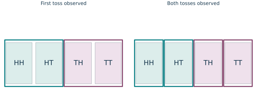
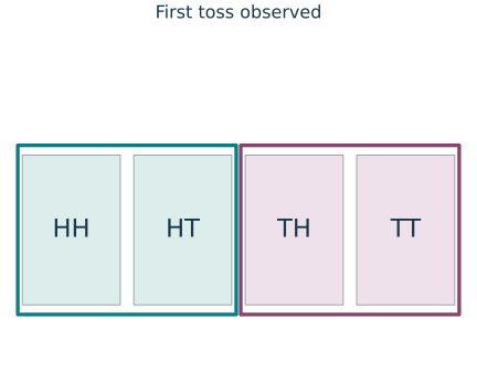
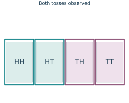
Observing the second toss refines two information blocks into four singleton blocks.
For a collection \(\mathcal C\subseteq2^\Omega\), the \(\sigma\)-algebra generated by \(\mathcal C\) is \[\sigma(\mathcal C) = \bigcap\{\mathcal A:\mathcal A\text{ is a $\sigma$-algebra and } \mathcal C\subseteq\mathcal A\}.\] It is the smallest \(\sigma\)-algebra containing \(\mathcal C\).
Definition. The intersection in this definition is a \(\sigma\)-algebra, so the smallest one really exists. In Euclidean space, the Borel \(\sigma\)-algebra is \[\gB(\R^d)=\sigma\{O:O\subseteq\R^d\text{ is open}\}.\]
Included sets. It contains all open and closed sets, intervals, rectangles, and every set obtained from these by countably many unions, intersections, and complements.
Default target. Unless stated otherwise, random vectors taking values in \(\R^d\) use \(\gB(\R^d)\) as their target \(\sigma\)-algebra.
Proof route. Exercise 11(1) proves that the intersection really is the smallest \(\sigma\)-algebra; see its solution.
As an informal working rule, Borel sets are the de facto sets in Euclidean space that we use for observations and events. They include open and closed sets and remain Borel under countable unions, intersections, and complements, but they do not include every subset of \(\R^d\). This is a useful middle ground between just intervals and all possible subsets.1
Sets such as \((a,b]\) and \([a,b]\) are Borel. In \(\R^d\), the rectangles \[(a_1,b_1]\times\cdots\times(a_d,b_d] =\prod_{j=1}^d(a_j,b_j]\] are Borel as well, and these rectangles generate \(\gB(\R^d)\).
The same Borel \(\sigma\)-algebra on \(\R\) is generated by any of the following collections: \[\{(-\infty,a]:a\in\R\},\qquad \{(a,b]:a<b\},\qquad \{(a,b):a<b\}.\] It is enough to restrict the endpoints to rational numbers when open intervals are used. For instance, \[(a,b)= \bigcup_{\substack{r,s\in\Q\\a<r<s<b}}(r,s),\] and the union is countable. These equivalent generators are useful because measurability needs to be checked only on a generating class. The countable-basis and rectangle steps are proved in Exercise 5; the generating-class test for functions is proved in Exercise 11.
Set limits are also written as \[\liminf_{n\to\infty} A_n =\bigcup_{m=1}^{\infty}\bigcap_{n\ge m}A_n, \qquad \limsup_{n\to\infty} A_n =\bigcap_{m=1}^{\infty}\bigcup_{n\ge m}A_n.\] The first is the event that all but finitely many \(A_n\) occur; the second is the event that infinitely many \(A_n\) occur. Both are measurable whenever all \(A_n\) are measurable.
A useful limiting-set picture.
Construction. If \(a<b_n<b\) and \(b_n\uparrow b\), then \[(a,b)=\bigcup_{n=1}^{\infty}(a,b_n].\]
Endpoint matters. This is a concrete reason to want countable unions: the limiting interval is still measurable. The endpoint matters—if we allowed \(b_n=b\), the union instead contains \(b\) and equals \((a,b]\).
Proof route. The membership arguments for this identity and the two set limits appear in Exercise 9.
3. Measures and probability measures
The length of \((a,b]\) is \(b-a\), and the volume of a rectangle \(\prod_{j=1}^d(a_j,b_j]\) is \(\prod_{j=1}^d(b_j-a_j)\). A measure extends this familiar idea of size to sets in an abstract measurable space.
Let \((\Omega,\F)\) be a measurable space. A function \(\nu:\F\to[0,\infty]\) is a measure if:
\(\nu(\emptyset)=0\); and
for every pairwise disjoint sequence \(A_1,A_2,\ldots\in\F\), \[\nu\left(\bigcup_{n=1}^{\infty}A_n\right) = \sum_{n=1}^{\infty}\nu(A_n).\]
The triple \((\Omega,\F,\nu)\) is a measure space. If \(\nu(\Omega)=1\), then \(\nu\) is a probability measure, usually denoted by \(P\), and \((\Omega,\F,P)\) is a probability space.
Countable additivity yields the following rules that are used constantly.
Let \(\nu\) be a measure.
If \(A\subseteq B\), then \(\nu(A)\leq\nu(B)\).
For arbitrary \(A_1,A_2,\ldots\in\F\), \[\nu\left(\bigcup_{n=1}^{\infty}A_n\right) \leq \sum_{n=1}^{\infty}\nu(A_n).\]
If \(A_n\uparrow A\), meaning \(A_1\subseteq A_2\subseteq\cdots\) and \(A=\bigcup_nA_n\), then \[\nu(A_n)\uparrow\nu(A).\]
If \(A_n\downarrow A\) and \(\nu(A_1)<\infty\), then \[\nu(A_n)\downarrow\nu(A).\]
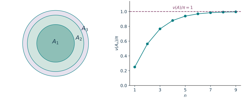
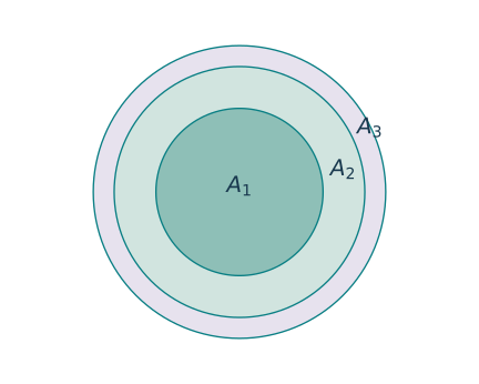
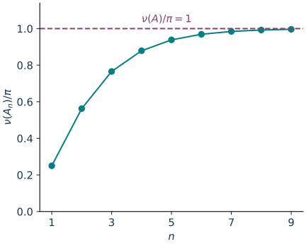
For disks \(A_n\) of radius \(1-2^{-n}\), \(m_2(A_n)=\pi(1-2^{-n})^2\uparrow\pi\). The finite drawing illustrates an infinite sequence.
Proof. For monotonicity, write \(B=A\cup(B\setminus A)\) as a disjoint union. For countable subadditivity, replace \(A_n\) by the disjoint sets \[B_1=A_1,\qquad B_n=A_n\setminus\bigcup_{j<n}A_j,\quad n\ge2.\] Then \(\bigcup_nB_n=\bigcup_nA_n\) and \(\nu(B_n)\le\nu(A_n)\).
For continuity from below, use the disjoint increments \(B_1=A_1\) and \(B_n=A_n\setminus A_{n-1}\). Countable additivity gives \[\nu(A)=\sum_{n=1}^{\infty}\nu(B_n) =\lim_{m\to\infty}\sum_{n=1}^m\nu(B_n) =\lim_{m\to\infty}\nu(A_m).\] For continuity from above, apply continuity from below to \(A_1\setminus A_n\uparrow A_1\setminus A\) and subtract from \(\nu(A_1)\). The finiteness of \(\nu(A_1)\) prevents the undefined subtraction \(\infty-\infty\). ◻
For \(x\in\Omega\), the Dirac measure at \(x\) is \[\delta_x(A)=\mathbf 1\{x\in A\}.\]
On a countable set with all subsets measurable, the counting measure is \(\nu_{\mathrm{count}}(A)=|A|\), allowing the value \(\infty\).
The Lebesgue measure \(m\) on \((\R,\gB(\R))\) is the unique translation-invariant Borel measure normalized by \[m((a,b])=b-a,\qquad -\infty<a<b<\infty.\]
Length as a probability.
Construction. Restricting Lebesgue measure to \([0,1]\) gives a probability measure, since \(m([0,1])=1\). Its measurable sets form the trace \(\sigma\)-algebra \[\gB_{[0,1]}=\{[0,1]\cap B:B\in\gB(\R)\}.\]
Interpretation. This is the familiar uniform probability on \([0,1]\): the probability of an interval inside \([0,1]\) is its length.
Inherited properties. The trace collection inherits countable unions and complements relative to \([0,1]\), and countable additivity is inherited from \(m\).
Discrete. Discrete probability measures are weighted sums of Dirac measures: \[P=\sum_{k=1}^{\infty}p_k\delta_{x_k}, \qquad p_k\ge0,\qquad \sum_{k=1}^{\infty}p_k=1.\]
Density. An absolutely continuous probability measure on \(\R\) takes the familiar form \(P(A)=\int_A f(x)\,dx\) for a nonnegative density \(f\) satisfying \(\int f=1\). Lecture 3 will unify both formulas as integration with respect to a measure.
Justification. Exercise 3 verifies the discrete construction, including the interchange of its two nonnegative sums. The existence and uniqueness of Lebesgue measure and the density characterization are covered by the measure-construction references.
Cumulative distribution functions.
Definition and properties. For a probability measure \(P\) on \((\R,\gB(\R))\), define \[F(x)=P((-\infty,x]).\] Then \(F\) is nondecreasing and right-continuous, with \(F(x)\to0\) as \(x\to-\infty\) and \(F(x)\to1\) as \(x\to\infty\).
Converse. Conversely, every function having these four properties determines a unique probability measure on \(\gB(\R)\), with \[P((a,b])=F(b)-F(a).\]
Existence. Thus a CDF always exists, even when neither a probability mass function nor a Lebesgue density exists.
Random vector. For a random vector with law \(P_X\) on \(\R^d\), the same idea gives \[F(x_1,\ldots,x_d) =P_X\bigl((-\infty,x_1]\times\cdots\times(-\infty,x_d]\bigr).\] This is the multivariate cumulative distribution function.
Proof route. The forward properties of a CDF are proved in Exercise 12. For the converse existence and uniqueness assertion, see the cited construction and inverse-CDF proofs.
Extra condition. The four one-dimensional conditions alone are not a multivariate characterization; rectangle increments must also be nonnegative.
Sigma-finiteness.
Definition. A measure \(\nu\) is \(\sigma\)-finite if \[\Omega=\bigcup_{n=1}^{\infty}E_n \quad\text{for measurable }E_n\text{ with }\nu(E_n)<\infty.\]
Examples and use. Probability measures, Lebesgue measure on \(\R^d\), and counting measure on a countable set are \(\sigma\)-finite. This mild condition supports the product and Radon–Nikodym theorems used later.
Covers. Concrete covers are the whole space for a probability measure, \([-n,n]^d\) for Lebesgue measure, and finite initial segments of an enumeration for a countable space.
Product measures.
Measurable sets. For measurable spaces \((\Omega_i,\F_i)\), define \[\F_1\otimes\F_2 = \sigma\{A_1\times A_2:A_i\in\F_i\}.\]
Measure. If \(\nu_1\) and \(\nu_2\) are \(\sigma\)-finite measures, there is a unique product measure \(\nu_1\otimes\nu_2\) satisfying \[(\nu_1\otimes\nu_2)(A_1\times A_2) = \nu_1(A_1)\nu_2(A_2).\]
Extension. The theorem says much more than the rectangle formula: it extends that formula consistently to every event in the product \(\sigma\)-algebra. Lecture 3 will use the product measure in Tonelli’s and Fubini’s theorems.
Proof route. The general existence/uniqueness proof is in the product-measure reference; Exercise 7 works out the finite case and contrasts it with dependent coordinates.
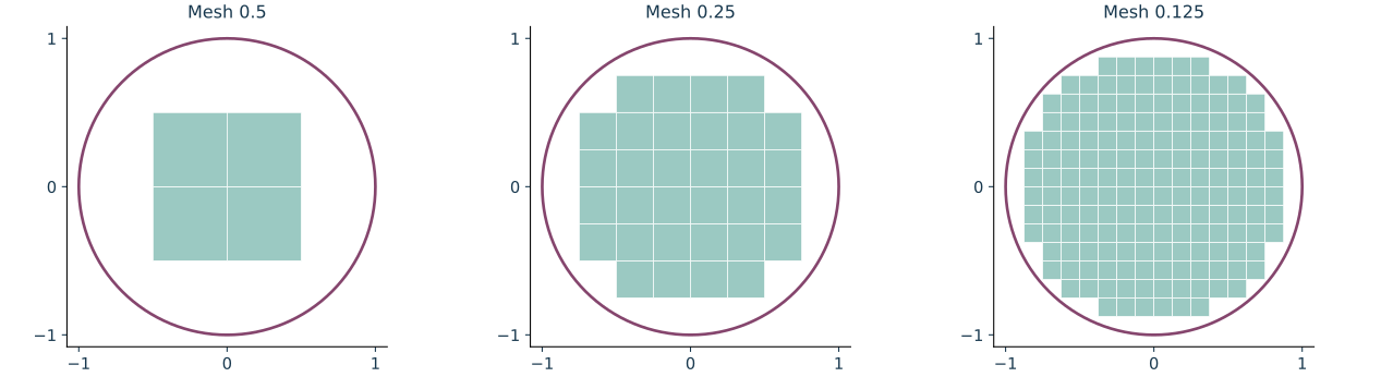
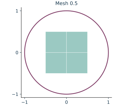
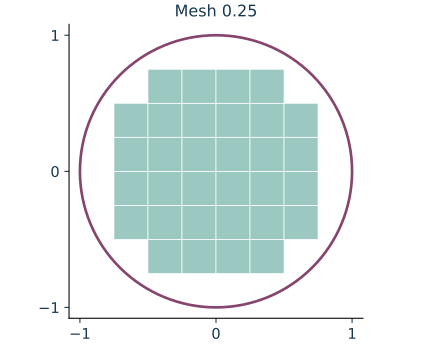
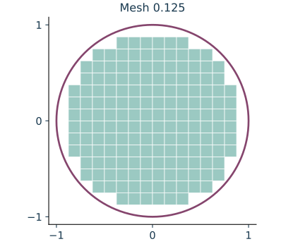
Rectangles generate the product sigma-algebra; sets in that sigma-algebra need not themselves be rectangles. The squares approximate the open disk from inside.
4. Measurable functions, random variables, and laws
Let \(\Omega\) be a set. A collection \(\F\subseteq 2^\Omega\) is a \(\sigma\)-algebra if:
\(\Omega\in\F\);
\(A\in\F\) implies \(A^c=\Omega\setminus A\in\F\); and
\(A_1,A_2,\ldots\in\F\) implies \(\bigcup_{n=1}^{\infty}A_n\in\F\).
The pair \((\Omega,\F)\) is a measurable space, and the elements of \(\F\) are called measurable sets. In probability, they are called events.
Familiar class. The next step is to broaden our familiar class of continuous functions.
Method. The useful idea is to express a condition on a function in terms of the sets it pulls back.
Reason. This is why inverse images are the central device.
For a map \(f:\Omega\to\Lambda\) and a set \(B\subseteq\Lambda\), the inverse image is \[f^{-1}(B)=\{\omega\in\Omega:f(\omega)\in B\}.\] Inverse images preserve the set operations used by \(\sigma\)-algebras: \[\begin{split} f^{-1}(B^c)&=(f^{-1}(B))^c,\\ f^{-1}\left(\bigcup_nB_n\right)&=\bigcup_nf^{-1}(B_n),\\ f^{-1}\left(\bigcap_nB_n\right)&=\bigcap_nf^{-1}(B_n). \end{split}\]
Let \((\Omega,\F)\) and \((\Lambda,\gG)\) be measurable spaces. A map \(f:\Omega\to\Lambda\) is \((\F,\gG)\)-measurable if \[f^{-1}(B)\in\F\qquad\text{for every }B\in\gG.\]
Criterion. It is enough to verify inverse images on a class that generates \(\gG\). In particular, a real-valued \(f\) is measurable if and only if \[\{\omega:f(\omega)\le a\}\in\F \qquad\text{for every }a\in\R.\]
Use. This is often the most useful calculation-based test.
Proof route. Exercise 11(2) proves the generating-class test; the solution explains why half-lines suffice.
In Euclidean space, the Borel \(\sigma\)-algebra is \[\gB(\R^d)=\sigma\{O:O\subseteq\R^d\text{ is open}\}.\] It contains all open and closed sets, intervals, rectangles, and every set obtained from these by countably many unions, intersections, and complements. Unless stated otherwise, random vectors taking values in \(\R^d\) use \(\gB(\R^d)\) as their target \(\sigma\)-algebra.
Let \((\Omega,\F)\) and \((\Lambda,\gG)\) be measurable spaces. A map \(f:\Omega\to\Lambda\) is \((\F,\gG)\)-measurable if \[f^{-1}(B)\in\F\qquad\text{for every }B\in\gG.\]
Borel functions in practice.
Meaning. For maps between Euclidean spaces, a Borel function means a measurable function when both spaces carry their Borel \(\sigma\)-algebras.
Convention. Unless specified otherwise, transformations used below are Borel measurable.
Continuous case. A continuous function pulls open sets back to open sets, which explains why continuous functions are Borel measurable.
Every continuous \(f:\R^d\to\R^k\) is Borel measurable.
If \(f:(\Omega,\F)\to(\Lambda,\gG)\) and \(g:(\Lambda,\gG)\to(\Xi,\gH)\) are measurable, then \(g\circ f\) is measurable.
If \(f\) and \(g\) are real-valued measurable functions, then \(f+g\), \(fg\), \(\min(f,g)\), and \(\max(f,g)\) are measurable.
If \(f_1,f_2,\ldots\) are extended real-valued measurable functions, then \(\inf_nf_n\), \(\sup_nf_n\), \(\liminf_nf_n\), and \(\limsup_nf_n\) are measurable.
These claims follow from inverse-image identities or composition with continuous maps. The worked supremum identity is left to the complete solution in Section 6. Complete proofs of the composition and arithmetic steps appear in Exercise 11; the countable supremum/infimum steps, including infinite values, appear in Exercise 4.
Closure. Composition retains a familiar property of continuous functions; closure under countable suprema and pointwise limits is an additional advantage of measurable functions.
Example. The rational-point indicators in Section 1.2 illustrate that measurability survives even when Riemann integrability does not.
Caveat. They do not give an example of continuous functions losing continuity: the finite-point indicators already have discontinuities.
On a probability space \((\Omega,\F,P)\), a random variable is a measurable map \[X:(\Omega,\F)\longrightarrow(\R,\gB(\R)).\] A measurable map into \((\R^d,\gB(\R^d))\) is a random vector.
These maps turn a potentially complicated sample space into numerical observations. The abbreviation “r.v.” means random variable; informally, the term is sometimes also used for random vectors.
Let \((\Omega,\F)\) be a measurable space. A function \(\nu:\F\to[0,\infty]\) is a measure if:
\(\nu(\emptyset)=0\); and
for every pairwise disjoint sequence \(A_1,A_2,\ldots\in\F\), \[\nu\left(\bigcup_{n=1}^{\infty}A_n\right) = \sum_{n=1}^{\infty}\nu(A_n).\]
The triple \((\Omega,\F,\nu)\) is a measure space. If \(\nu(\Omega)=1\), then \(\nu\) is a probability measure, usually denoted by \(P\), and \((\Omega,\F,P)\) is a probability space.
The law of a random variable \(X\) is the probability measure \[P_X=P\circ X^{-1}, \qquad P_X(B)=P(X\in B),\quad B\in\gB(\R).\] It is also denoted by \(\mathcal L(X)\) or \(\mu_X\).
Event notation. The notation \(P(X\in B)\) is shorthand for \(P(\{\omega:X(\omega)\in B\})\). Measurability is exactly what guarantees that this inverse image is an event to which \(P\) may be applied.
Justification. Why the law is a probability measure, and why \(P_{h(X)}=P_X\circ h^{-1}\), are verified in Exercise 11(4).
A finite inverse-image picture.
For a map \(f:\Omega\to\Lambda\) and a set \(B\subseteq\Lambda\), the inverse image is \[f^{-1}(B)=\{\omega\in\Omega:f(\omega)\in B\}.\]
The law of a random variable \(X\) is the probability measure \[P_X=P\circ X^{-1}, \qquad P_X(B)=P(X\in B),\quad B\in\gB(\R).\] It is also denoted by \(\mathcal L(X)\) or \(\mu_X\).
On \(\Omega=\{a,b,c,d\}\) with all subsets measurable and each outcome of probability \(1/4\), define the random variable \(X\) by \[\begin{array}{c|rrrr} \omega&a&b&c&d\\\hline X(\omega)&-1&0&0&2 \end{array}\] Choose a closed interval \(B=[\ell,r]\) with integer endpoints \(-2\le\ell\le r\le3\). Which outcomes belong to \(X^{-1}(B)\), and how much probability does \(P_X\) assign to \(B\)? Compare a singleton interval with an interval that contains none of the observed values.
Explore an inverse image
✓ marks an outcome in the inverse image.
B = [0, 0]; X⁻¹(B) = {b, c}; P_X(B) = 0.5.
Direction. The map \(X\) sends outcomes to numbers. An inverse image instead pulls a set of numbers back to outcomes.
Probability. Add the probabilities of those outcomes to obtain \(P_X(B)=P(X^{-1}(B))\); repeated values of \(X\) collect multiple masses.
Caveat. No inverse function is needed, and a nonempty interval can have an empty inverse image.
For \(B=[0,0]=\{0\}\), the inverse image is \(\{b,c\}\) and \(P_X(B)=1/4+1/4=1/2\). For \(B=[3,3]\), it is empty and \(P_X(B)=0\). These are exact finite probabilities, not simulation estimates.
For \((X,Y)=(\cos U,\sin U)\), the law \(P_{(X,Y)}\) is the pushforward of the uniform law on \([0,2\pi)\). If \(S=\{(x,y):x^2+y^2=1\}\), then \[P_{(X,Y)}(S)=1 \quad\text{but}\quad m_2(S)=0,\] where \(m_2\) is two-dimensional Lebesgue measure. If a Lebesgue density existed, its integral over \(S\) would be zero, a contradiction. The law exists; only a particular representation of it as a two-dimensional density fails. For the area-zero calculation and the rectangle-identity argument, return to Exercise 6.
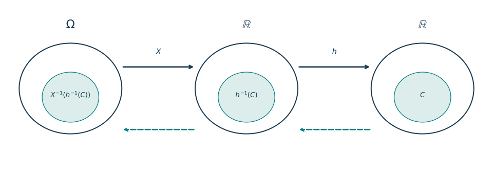
Maps carry outcomes forward; inverse images pull events back into the original sample space.
If \(X=(X_1,\ldots,X_d)\) is a random vector and \(h:\R^d\to\R^k\) is Borel measurable, then \(h(X)\) is a random vector. This single statement validates familiar constructions such as \[\bar X_n=\frac1n\sum_{i=1}^nX_i,\qquad \max_{1\le i\le n}X_i,\qquad \|X\|_2,\qquad \mathbf 1\{X\in B\}.\] The law of \(h(X)\) can be written as another pushforward: \[P_{h(X)}=P_X\circ h^{-1}.\] This viewpoint separates two objects that are often conflated:
\(X\) is a function on the original sample space; and
\(P_X\) is a probability measure on the observation space.
Most statistical calculations depend only on \(P_X\), but almost-sure comparisons between several random variables depend on how they are jointly defined on \(\Omega\).
The point of the abstraction is to find a useful mathematical workspace in which our operations are rigorous. We want familiar sets such as intervals, closure under countable operations, and functions that preserve measurable events. Borel sets and Borel measurable functions are the standard starting point. This is not a blanket objection to using all subsets: on a finite or countable sample space that is natural. In Euclidean space, however, ordinary length cannot be extended to every subset while retaining both countable additivity and translation invariance. The Vitali-set reference gives the precise obstruction; its set-theoretic construction is optional.
5. Technical extensions and further reading
Low priority — not examined: Completion and null-set modifications
The Borel \(\sigma\)-algebra is generated by topology, but it is not complete with respect to Lebesgue measure: a subset of a Borel null set need not itself be Borel. The Lebesgue \(\sigma\)-algebra is the completion of \(\gB(\R^d)\) under Lebesgue measure. It contains every set of the form \[B\cup N,\qquad B\in\gB(\R^d),\quad N\subseteq Z,\quad Z\in\gB(\R^d),\quad m(Z)=0.\] The completed measure assigns \(N\) measure zero.
Completion formalizes the principle that changing an object on a null set should not affect its integral or probability. It also explains why one must specify the relevant \(\sigma\)-algebra when using the phrase “measurable function”: Borel measurability and Lebesgue measurability are closely related but not identical.
An informal picture of completion.
Completion allows all changes to measurable sets on sets of measure zero. For real-valued functions on \(\R^d\), keeping the target Borel \(\sigma\)-algebra fixed, this gives the hierarchy \[\{\text{Borel measurable functions}\} \subseteq\{\text{Lebesgue measurable functions}\}.\]
Optional size comparison.
For \(d\geq1\), the Borel sets have the same cardinality as \(\R\), whereas the collection of all subsets of \(\R^d\) has strictly larger cardinality: \[|\gB(\R^d)|=|\R|<|2^{\R^d}|.\] Thus some subsets are not Borel. There are even non-Borel subsets of Borel null sets, which completion makes measurable. The set-theoretic argument is optional; see Tao’s An Introduction to Measure Theory, Exercise 1.4.16. For the full completion construction, see the proof reference; Exercise 8 checks what happens to subsets of a null set. Return to the core Borel definition.
Low priority — not examined: Infinite products and random measures
Finite product measures are not by themselves a construction of an infinite sequence \(X_1,X_2,\ldots\). For finite-state or Euclidean coordinate spaces, the Kolmogorov extension theorem gives an infinite-dimensional probability measure when a consistent family of finite-dimensional distributions is supplied. This is the rigorous foundation for canonical sequence and stochastic-process models. The space assumptions and proof are stated in the extension-theorem reference.
A measure can itself also be data. Let \(Y_n\) be a symmetric random matrix, and write its eigenvalues as \(\lambda_1,\ldots,\lambda_n\). Its empirical spectral distribution is the random probability measure \[\mu_{Y_n}=\frac1n\sum_{i=1}^n\delta_{\lambda_i}.\] For a normalized Gaussian orthogonal ensemble, this random measure converges under suitable conditions to the semicircle law with density \[x\longmapsto \frac{1}{2\pi}\sqrt{4-x^2}\, \mathbf 1\{|x|\le2\}.\] The density is interpreted as zero outside \([-2,2]\), as in the piecewise formula in the introductory preview. This example motivates later notions of weak convergence for measures; see [5].
Return to the core definition of a law.
Further reading: References, construction theorems, and self-study
For a probability-oriented development of measurable spaces, measures, and measurable maps, see Chapters 1–2 of [1]. Sections 1.1–1.2 of [4] emphasize the statistical viewpoint. A more analysis-centered treatment, including construction and completion of Lebesgue measure, appears in [3].
Useful self-study directions are:
the Carathéodory extension theorem, which constructs a measure from its values on a simpler class of sets;
the monotone-class and \(\pi\)–\(\lambda\) theorems, which reduce equality and measurability checks to generators;
the Kolmogorov extension theorem for stochastic processes; and
random probability measures and empirical distributions.
Key ideas
A sigma-algebra specifies which sets can be assigned probabilities.
Countable additivity yields monotonicity, subadditivity and continuity of measures.
Random variables are measurable maps; their laws live on the value space.
One measure-theoretic language includes discrete, continuous and singular models.
Looking ahead
Lecture 3 builds integrals from the measures introduced here. It then asks when a limit or a change in integration order preserves the answer. Continue to Lecture 3.
6. Exercises and complete solutions12 exercises · complete solutions
The solution links in the main text lead directly to the relevant analysis below. Exercises 9–12 give additional justifications; Section 6.2 provides precise references for longer construction theorems.
Let \(\F\) be a \(\sigma\)-algebra on \(\Omega\).
Prove that \(\F\) is closed under countable intersections and set differences.
Let \(\Omega=\{1,2,3,4,5,6\}\) and \(A=\{1,3,5\}\). Find \(\sigma(\{A\})\), the smallest \(\sigma\)-algebra containing \(A\).
Is \(\{1,2\}\) measurable with respect to \(\sigma(\{A\})\)? Interpret the answer in terms of information.
Reveal solution
For \(A_n\in\F\), each \(A_n^c\) belongs to \(\F\), and hence \[\bigcap_{n=1}^{\infty}A_n = \left(\bigcup_{n=1}^{\infty}A_n^c\right)^c \in\F.\] For \(A,B\in\F\), \(A\setminus B=A\cap B^c\in\F\).
A \(\sigma\)-algebra containing \(A\) must also contain \(A^c\), \(\emptyset\), and \(\Omega\). The collection \[\{\emptyset,\Omega,A,A^c\} = \{\emptyset,\Omega,\{1,3,5\},\{2,4,6\}\}\] is itself a \(\sigma\)-algebra, so it is \(\sigma(\{A\})\). The set \(\{1,2\}\) is not in this collection. Observing only whether the outcome lies in \(A\) distinguishes odd from even outcomes, but it does not reveal the exact outcome.
Let \(X_1,X_2,\ldots\) be independent fair coin tosses, with \(X_i=1\) for heads. Define \[A_n=\{\text{at least one head occurs among the first }n\text{ tosses}\}.\]
Show that \(A_n\uparrow A\), where \(A\) is the event that a head occurs at some finite time.
Compute \(P(A_n)\) and use continuity from below to find \(P(A)\).
Find the probability that all tosses are tails.
Reveal solution
If a head appears among the first \(n\) tosses, it also appears among the first \(n+1\), so \(A_n\subseteq A_{n+1}\). The union \(\bigcup_nA_n\) is exactly the event that a head appears at some finite index; hence \(A_n\uparrow A\). Independence gives \[P(A_n)=1-P(X_1=\cdots=X_n=0)=1-2^{-n}.\] By continuity from below, \[P(A)=\lim_{n\to\infty}P(A_n)=1.\] The event that all tosses are tails is \(A^c\), so it has probability zero. A probability-zero event need not be the empty set.
Let \(x_1,x_2,\ldots\) be distinct points of \(\R\), and let \(p_k\ge0\) satisfy \(\sum_{k=1}^{\infty}p_k=1\). Define \[\mu(A)=\sum_{k=1}^{\infty}p_k\mathbf 1\{x_k\in A\}, \qquad A\in\gB(\R).\]
Show that \(\mu\) is a probability measure.
Express \(\mu\) using Dirac measures.
Write its CDF.
Explain why the same additivity argument gives counting measure on a countable sample space.
Reveal solution
Clearly \(\mu(\emptyset)=0\) and \(\mu(\R)=\sum_kp_k=1\). If \(A_1,A_2,\ldots\) are pairwise disjoint, then for each fixed \(k\) the point \(x_k\) belongs to at most one \(A_j\). Since all terms are nonnegative, \[\begin{split} \mu\left(\bigcup_{j=1}^{\infty}A_j\right) &=\sum_{k=1}^{\infty}p_k \sum_{j=1}^{\infty}\mathbf 1\{x_k\in A_j\}\\ &=\sum_{j=1}^{\infty} \sum_{k=1}^{\infty}p_k\mathbf 1\{x_k\in A_j\} =\sum_{j=1}^{\infty}\mu(A_j). \end{split}\] Here the interchange needs no integration theorem: for numbers \(a_{jk}\geq0\), both iterated sums equal \[\sup_{J,K}\sum_{j=1}^J\sum_{k=1}^K a_{jk}.\] Indeed, every finite choice of indices is contained in such a finite rectangle, and nonnegativity makes all these partial sums increase. The same reasoning allows the value \(+\infty\). Thus \(\mu\) is countably additive and is a probability measure. It can be written as \[\mu=\sum_{k=1}^{\infty}p_k\delta_{x_k},\] and its CDF is \[F(t)=\mu((-\infty,t]) =\sum_{k=1}^{\infty}p_k\mathbf 1\{x_k\le t\}.\] Putting unit weight on every point instead gives counting measure; the additivity calculation is unchanged, although the total mass can now be infinite. A single point with weight one gives the Dirac measure.
Let \(X_1,X_2,\ldots\) be real-valued random variables.
Prove directly from inverse images that \(M_n=\max_{1\le i\le n}X_i\) is a random variable.
Prove that \(\limsup_{n\to\infty}X_n\) is an extended real-valued measurable function.
Reveal solution
For every \(a\in\R\), \[\{M_n\le a\}=\bigcap_{i=1}^n\{X_i\le a\}\in\F,\] so the half-line criterion shows that \(M_n\) is measurable.
Write \[\limsup_{n\to\infty}X_n = \inf_{m\ge1}\sup_{n\ge m}X_n.\] For a countable family of measurable functions, \[\left\{\sup_{n\ge m}X_n\le a\right\} = \bigcap_{n\ge m}\{X_n\le a\}\in\F,\] so each \(\sup_{n\ge m}X_n\) is measurable. For an infimum the convenient identity uses a strict inequality: \[\{\inf_jY_j<a\}=\bigcup_j\{Y_j<a\},\qquad \{\inf_jY_j\leq a\} =\bigcap_{k=1}^{\infty}\bigcup_j\{Y_j<a+1/k\}.\] Each \(\{Y_j<b\}\) is measurable because it is the union of \(\{Y_j\leq r\}\) over rational \(r<b\). Thus countable infima are measurable, and applying this to \(Y_m=\sup_{n\geq m}X_n\) proves the limsup claim. The formula \(\liminf_nX_n=\sup_m\inf_{n\geq m}X_n\) proves the corresponding liminf assertion. These identities hold for extended real values as well; for example, \(\{Y=+\infty\}=\bigcap_{k\geq1}\{Y>k\}\) is measurable. One cannot replace the strict inequality above by \(\{\inf_jY_j\leq a\}=\bigcup_j\{Y_j\leq a\}\): take \(Y_j=a+1/j\).
Let \(\mathcal C=\{(-\infty,a]:a\in\R\}\). Show that \(\sigma(\mathcal C)=\gB(\R)\). Then prove that open sets in \(\R^d\) are countable unions of rational open boxes, and that either bounded closed boxes or bounded half-open boxes generate \(\gB(\R^d)\).
Reveal solution
Each \((-\infty,a]\) is closed, hence Borel, so \(\sigma(\mathcal C)\subseteq\gB(\R)\). Conversely, \[(a,b] = (-\infty,b]\setminus(-\infty,a] \in\sigma(\mathcal C).\] Also, \[(a,b) = \bigcup_{\substack{q\in\Q\\a<q<b}}(a,q],\] which is a countable union of sets in \(\sigma(\mathcal C)\). Every open subset of \(\R\) is a countable union of bounded open intervals with rational endpoints, so every open set belongs to \(\sigma(\mathcal C)\). Since open sets generate \(\gB(\R)\), we have \(\gB(\R)\subseteq\sigma(\mathcal C)\).
Here is the countable-basis step in any dimension. Given \(x\) in an open set \(O\), an open ball around \(x\) is contained in \(O\). Choose rational endpoints \(r_j<x_j<s_j\) so close to \(x_j\) that the closed box \(\prod_j[r_j,s_j]\) lies in that ball. Thus the rational open boxes contained in \(O\) cover \(O\), as do the rational closed boxes contained in \(O\). There are only countably many such boxes because each is specified by \(2d\) rational numbers. Hence closed boxes generate every open set and therefore the Borel sets; the reverse inclusion holds because closed boxes are Borel.
Half-open boxes are Borel as well, since \[\prod_{j=1}^d(a_j,b_j] =\bigcap_{m=1}^{\infty}\prod_{j=1}^d(a_j,b_j+1/m).\] Conversely, every open box \(\prod_j(a_j,b_j)\) is the union, over all sufficiently large \(m\), of the half-open boxes \(\prod_j(a_j,b_j-1/m]\). This proves the other generating claim. It also justifies restricting to rational endpoints in the open-interval generators on \(\R\).
Let \(U\sim\Unif[0,2\pi)\) and \(Z=(\cos U,\sin U)\).
Show that every point has probability zero and that the circle \(S=\{z:\|z\|_2=1\}\) has two-dimensional Lebesgue measure zero. For the latter, cover the circle by \(N\) small squares.
Deduce that the law has no discrete mass-function representation and is not absolutely continuous with respect to area.
Prove that no nonnegative Borel measurable density can satisfy Equation (1) for every rectangle. Explain why agreement on rectangles would imply agreement on \(S\).
Let \(B_\alpha=\{(\cos t,\sin t):0\le t\le\alpha\}\) for \(0\le\alpha\le2\pi\). Compute \(P_Z(B_\alpha)\).
Reveal solution
Points and area. The map \(t\mapsto(\cos t,\sin t)\) is one-to-one on \([0,2\pi)\), so the inverse image of a point is empty or a singleton. Uniform probability assigns it zero mass. To check the area assertion, put \(h=2\pi/N\) and \(t_k=kh\), \(0\leq k<N\). On \([t_k,t_k+h]\), the mean value theorem gives \(|\cos t-\cos t_k|\leq h\) and \(|\sin t-\sin t_k|\leq h\). The arc is therefore contained in the closed square centered at \((\cos t_k,\sin t_k)\) with side \(2h\). The \(N\) squares cover \(S\), so \[0\leq m_2(S)\leq N(2h)^2=\frac{16\pi^2}{N}\longrightarrow0.\] The set \(S\) is closed, hence Borel, so this proves \(m_2(S)=0\).
Consequences for the law. A discrete probability law must put total mass one on a countable set. Here every countable set has probability zero by countable additivity. Also \(P_Z(S)=1\) while \(m_2(S)=0\), so \(P_Z\not\ll m_2\): absolute continuity would require every area-zero set to have probability zero.
Why the rectangle equation fails. Suppose a function \(f\geq0\) satisfied Equation (1). Define the measure \(\nu_f(A)=\int_A f\,dm_2\) on Borel sets. We use two standard facts about Lebesgue integration: a nonnegative measurable function defines a measure this way, and an integral over a null set is zero. The iterated integral equals this area integral on rectangles by Tonelli’s theorem; see the integration and product references. For \(k\geq1\), the assumed equation gives \(\nu_f([-k,k]^2)=P_Z([-k,k]^2)=1\); continuity from below yields \(\nu_f(\R^2)=1\).
Now apply the following uniqueness fact: two finite measures with the same total mass that agree on a generating collection closed under finite intersections agree on the whole generated \(\sigma\)-algebra. Such a collection is called a \(\pi\)-system. Its proof is the finite-measure uniqueness theorem cited below. Here use bounded closed rectangles (including degenerate ones), together with \(\emptyset\) and \(\R^2\). These generate the Borel sets by Exercise 5. For a degenerate rectangle, the area integral is zero and its intersection with \(S\) contains at most two points, so its \(P_Z\)-mass is also zero. All the hypotheses are met. Consequently \(\nu_f=P_Z\) on Borel sets, but \[1=P_Z(S)=\nu_f(S)=\int_Sf\,dm_2=0,\] a contradiction. This supplies the step from rectangles to the curved support that is implicit in the main-text explanation.
Arc probabilities. Except for endpoints, which have probability zero, the event \(\{Z\in B_\alpha\}\) is \(\{0\le U\le\alpha\}\). Therefore \[P_Z(B_\alpha)=\frac{\alpha}{2\pi}.\] This is a one-dimensional uniform law along the circle, not a two-dimensional density. At \(\alpha=0\) the arc is one point and the probability is zero; at \(\alpha=2\pi\) it is the whole circle and the probability is one.
Let \(\nu\) be the Bernoulli\((p)\) measure on \(\{0,1\}\), where \(0\leq p\leq1\), so \(\nu(\{1\})=p\). On \(\{0,1\}^2\) use the product measure \(\nu\otimes\nu\). Let \(X_i(x_1,x_2)=x_i\) be the coordinate maps.
Compute the probability of every singleton \((x_1,x_2)\).
Compute \(P(X_1+X_2=1)\).
Explain where the product assumption enters.
Reveal solution
For \(x_1,x_2\in\{0,1\}\), the rectangle formula gives \[P((X_1,X_2)=(x_1,x_2)) =p^{x_1+x_2}(1-p)^{2-x_1-x_2}.\] Equivalently, the four masses are \((1-p)^2\), \(p(1-p)\), \(p(1-p)\), and \(p^2\) at \((0,0),(0,1),(1,0),(1,1)\), respectively. This list also covers \(p=0\) and \(p=1\) without needing to interpret \(0^0\) in the compact formula. Hence \[P(X_1+X_2=1) =P(1,0)+P(0,1)=2p(1-p).\] The multiplication of marginal probabilities is exactly the defining rectangle property of the product measure. A general joint measure with the same Bernoulli marginals need not assign these probabilities and need not make \(X_1\) and \(X_2\) independent. For example, setting \(X_1=X_2=W\) for one Bernoulli\((p)\) variable gives the same two marginals but \(P(X_1+X_2=1)=0\). For \(0<p<1\) this differs from the independent answer.
Low priority — not examined: Optional practice: completion
Let \((\Omega,\F,\nu)\) be a measure space and let \(N\in\F\) satisfy \(\nu(N)=0\). Define the completion \[\overline{\F} = \{A\cup M:A\in\F,\ M\subseteq N_A \text{ for some }N_A\in\F\text{ with }\nu(N_A)=0\}.\] Explain why every subset \(M\subseteq N\) belongs to \(\overline{\F}\) and why its completed measure must be zero.
Reveal solution
Take \(A=\emptyset\) and \(N_A=N\). Then \(M=\emptyset\cup M\) has the required representation, so \(M\in\overline{\F}\). Any extension that remains monotone must satisfy \[0\le\overline{\nu}(M)\le\overline{\nu}(N)=\nu(N)=0.\] Thus \(\overline{\nu}(M)=0\). The completion adds all such subsets while leaving the measure of every original event unchanged. The separate tasks of proving that \(\overline\F\) is a \(\sigma\)-algebra and that the extension is well-defined are supplied by the completion theorem and its proof.
6.1. Further justification exercises
Explain why \(\liminf_n A_n\) consists of points in all sufficiently late \(A_n\), whereas \(\limsup_n A_n\) consists of points in infinitely many \(A_n\). If \(a<b_n<b\) and \(b_n\uparrow b\), prove \(\bigcup_n(a,b_n]=(a,b)\).
On \(\Omega=\{0,1\}^{\mathbb N}\), let \(X_i(\omega)=\omega_i\) and \(S_n=n^{-1}\sum_{i=1}^nX_i\). Use the \(\sigma\)-algebra generated by events specifying a finite initial segment. Show that \[\{\liminf_n S_n>1/3\} =\bigcup_{\substack{r\in\Q\\r>1/3}}\ \bigcup_{N=1}^{\infty}\ \bigcap_{n\geq N}\{S_n>r\},\] and deduce measurability.
Explain why no fixed finite initial segment determines membership in this event.
Reveal solution
Set limits. Membership in \(\bigcup_N\bigcap_{n\geq N}A_n\) means that some \(N\) works for every later \(n\); membership in \(\bigcap_N\bigcup_{n\geq N}A_n\) means that every \(N\) has a later successful \(n\). These are exactly “eventually always” and “infinitely often.” For the intervals, every point in the union lies strictly between \(a\) and \(b\). Conversely, if \(a<x<b\), convergence \(b_n\to b\) implies \(b_n>x\) for some \(n\), so \(x\in(a,b_n]\). If a nondecreasing sequence reaches \(b\), the union instead includes \(b\).
The limiting event. If \(\liminf_n S_n>1/3\), choose a rational \(r\) strictly between these two numbers. By the definition \(\liminf_n S_n=\sup_N\inf_{n\geq N}S_n\), some tail has infimum greater than \(r\), so all its \(S_n\) exceed \(r\). Conversely, if eventually \(S_n>r\) for some \(r>1/3\), then \(\liminf_n S_n\geq r>1/3\). Notice the weak inequality in this converse: a sequence strictly above \(r\) can converge to \(r\).
For each \(n\), the set \(\{S_n>r\}\) is a finite union of events specifying the first \(n\) zeros and ones: include exactly the strings whose average exceeds \(r\). It is therefore measurable. Both unions in the displayed identity and the intersection are countable, so the limiting event is measurable as well. This argument identifies an event; it does not yet calculate its probability. Existence of the infinite-sequence probability law is the separate construction cited in the infinite-product reference.
Why finite observations do not suffice. After any fixed initial segment, append zeros forever or append ones forever. In the first case \(S_n\to0\); in the second \(S_n\to1\). These two sequences agree on all the observed coordinates but give different answers to the limiting event. Countable set operations let us describe it without requiring a finite observation to decide it.
For an enumeration \(\{q_1,q_2,\ldots\}\) of \(\Q\cap[0,1]\), set \(f_n=\mathbf1_{\{q_1,\ldots,q_n\}}\). Prove the Riemann-integral assertions in Section 1.2, and compute the Lebesgue integral of the limit.
For \(g_n=\mathbf1_{[n,n+1]}\) on \(\R\), prove pointwise convergence to zero while \(\int g_n\,dm=1\). Explain why the sequence is not increasing and why no integrable function can dominate every \(g_n\).
Reveal solution
Finite rational sets and their limit. Every interval of positive length contains an irrational point, so every lower sum of \(f_n\) is zero. Given \(\epsilon>0\), enclose its finitely many nonzero points in small intervals of total length less than \(\epsilon\). Choose the endpoints away from those points and include them in a partition; use one-sided intervals at \(0\) or \(1\). Only these small intervals can contribute to the upper sum, so that sum is less than \(\epsilon\). The Darboux criterion gives \(\int_0^1f_n\,dx=0\).
Pointwise, \(f_n\uparrow f=\mathbf1_{\Q\cap[0,1]}\). Every nondegenerate partition interval contains both rational and irrational points, so \(f\) has upper sum \(1\) and lower sum \(0\) for every partition. Thus \(f\) is not Riemann integrable. For Lebesgue measure, a singleton can be enclosed in intervals of arbitrarily small length and hence has measure zero. Countable subadditivity gives \(m(\Q\cap[0,1])=0\). Therefore \[\int_0^1 f\,dm=m(\Q\cap[0,1])=0=\lim_n\int_0^1f_n\,dm.\] The limit has left the Riemann class, but the Lebesgue integrals do agree with the limit of the integrals in this example.
An escaping block. For any fixed \(x\), eventually \(n>x\), so \(g_n(x)=0\). Each interval \([n,n+1]\) has length one, giving \[\int \lim_n g_n\,dm=0\quad\hbox{but}\quad \lim_n\int g_n\,dm=1.\] At \(x=n+1/2\), \(g_n(x)=1\) and \(g_{n+1}(x)=0\), so the sequence is not increasing. If an integrable nonnegative \(g\) dominated every \(g_n\), it would satisfy \(g\geq1\) on \(\bigcup_{n\geq1}[n,n+1]=[1,\infty)\), which forces \(\int g\,dm=\infty\), a contradiction. The same argument works for domination almost everywhere: the union of the countably many exceptional null sets is still null.
These are the missing hypotheses for the monotone and dominated convergence theorems, respectively, which will be developed in Lecture 3. Fatou’s inequality would only assert \(0\leq1\) here and causes no contradiction. Their proofs are also available in [1] (Theorems 1.5.5, 1.5.7, and 1.5.8).
Prove that the intersection of all \(\sigma\)-algebras on \(\Omega\) containing \(\mathcal C\) is a \(\sigma\)-algebra and is the smallest one containing \(\mathcal C\).
If \(\gG=\sigma(\mathcal C)\), prove that \(f:(\Omega,\F)\to(\Lambda,\gG)\) is measurable whenever \(f^{-1}(C)\in\F\) for every \(C\in\mathcal C\). Deduce the half-line test for a real-valued function.
Prove that continuous maps between Euclidean spaces are Borel measurable, that compositions of measurable maps are measurable, and that the arithmetic operations in Proposition 2 preserve measurability.
Prove that \(P_X(B)=P(X^{-1}(B))\) is a probability measure and that \(P_{h(X)}(B)=P_X(h^{-1}(B))\) for measurable \(h\).
Reveal solution
1. The generated \(\sigma\)-algebra. The family being intersected is nonempty because \(2^\Omega\) belongs to it. Its intersection contains \(\Omega\) and \(\mathcal C\). If \(A\) belongs to every member of the family, so does \(A^c\); if each \(A_n\) belongs to every member, so does \(\bigcup_n A_n\). These observations prove the \(\sigma\)-algebra axioms. The intersection is contained in every \(\sigma\)-algebra containing \(\mathcal C\), which proves minimality.
2. Checking generators. Define \[\mathcal D=\{B\subseteq\Lambda:f^{-1}(B)\in\F\}.\] Since inverse images preserve the whole space, complements, and countable unions, \(\mathcal D\) is a \(\sigma\)-algebra on \(\Lambda\). The hypothesis says \(\mathcal C\subseteq\mathcal D\), so \(\gG=\sigma(\mathcal C)\subseteq\mathcal D\). This is exactly measurability of \(f\). By Exercise 5, the half-lines \((-\infty,a]\) generate \(\gB(\R)\); checking \(\{f\leq a\}\in\F\) for every \(a\in\R\) therefore suffices.
3. Continuous maps, compositions, and arithmetic. A continuous map has open inverse images of open sets. Open sets generate the Borel \(\sigma\)-algebra, so part 2 proves Borel measurability. For measurable \(f\) and \(h\), the identity \((h\circ f)^{-1}(B)=f^{-1}(h^{-1}(B))\) proves composition is measurable.
If \(f\) and \(g\) are real-valued measurable functions on \(\Omega\), the map \(F=(f,g)\) is measurable: the inverse image of a closed rectangle \([a,b]\times[c,d]\) is the intersection \(\{a\leq f\leq b\}\cap\{c\leq g\leq d\}\in\F\), and these rectangles generate \(\gB(\R^2)\) by Exercise 5. The maps \((u,v)\mapsto u+v,uv,\min(u,v),\max(u,v)\) are continuous. Composing each with \(F\) proves all four arithmetic claims. The same rectangle argument proves that a finite vector is measurable exactly when each coordinate is measurable; the reverse direction uses the continuous coordinate projections. Countable extrema and limits are handled separately in Exercise 4.
4. Pushing a probability measure forward. The empty set has empty inverse image, and the entire target has inverse image \(\Omega\), so \(P_X(\emptyset)=0\) and \(P_X(\R)=1\). For pairwise disjoint measurable \(B_j\), their inverse images are measurable and disjoint. Consequently \[P_X\Bigl(\bigcup_jB_j\Bigr) =P\Bigl(\bigcup_jX^{-1}(B_j)\Bigr) =\sum_jP(X^{-1}(B_j))=\sum_jP_X(B_j).\] Thus \(P_X\) is a probability measure. Finally, \[P_{h(X)}(B)=P((h\circ X)^{-1}(B)) =P(X^{-1}(h^{-1}(B)))=P_X(h^{-1}(B)),\] which proves the distribution formula used in the main text.
For a probability measure \(P\) on \((\R,\gB(\R))\), let \(F(x)=P(( -\infty,x])\). Prove monotonicity, right-continuity, the limits \(F(x)\to0\) as \(x\to-\infty\) and \(F(x)\to1\) as \(x\to\infty\), and \[P((a,b])=F(b)-F(a)\qquad(a<b).\] Identify where finiteness of the measure is used. Does this argument also construct a probability measure from a candidate \(F\)?
Reveal solution
If \(x\leq y\), then \((-\infty,x]\subseteq(-\infty,y]\), so monotonicity of \(P\) gives \(F(x)\leq F(y)\). If \(x_n\downarrow x\), the corresponding half-lines decrease to \((-\infty,x]\). Continuity from above applies because their probabilities are finite and gives \(F(x_n)\downarrow F(x)\). In particular \(F(x+1/n)\to F(x)\); monotonicity squeezes \(F(y)\) between \(F(x)\) and \(F(x+1/n)\) whenever \(x<y\leq x+1/n\). This proves right-continuity for arbitrary approaches from the right.
The sets \((-\infty,n]\) increase to \(\R\), while \((-\infty,-n]\) decrease to \(\emptyset\). Continuity from below and above, respectively, give \(F(n)\to1\) and \(F(-n)\to0\). Monotonicity extends these integer limits to the limits along all real \(x\). The decreasing-set steps use finiteness; the increasing-set step does not. Finally, \[(-\infty,b]=(-\infty,a]\ \dot\cup\ (a,b]\] is a disjoint union, so additivity gives the interval formula.
This proves the properties of the CDF of an existing measure. The converse is a separate existence theorem: every nondecreasing, right-continuous \(F\) with these two limiting values is the CDF of a probability measure. Its construction, and uniqueness from the half-line probabilities, are proved in the CDF and Stieltjes-measure references below.
6.2. References for longer proofs
The results used in the main sections keep their assigned priority. The references below supply longer proofs and construction details; they do not add new examination requirements. Exercises above give the local arguments students can work through with this lecture’s tools.
- Uniqueness from rectangles.
The \(\pi\)–\(\lambda\) theorem and measure uniqueness are proved in [1] (Theorems A.1.4–A.1.5); see the author’s fifth-edition text. The finite-measure version stated in Exercise 6 is the fact needed for Equation (1).
- Existence of measures and CDFs.
Durrett’s Theorem 1.1.4 constructs the unique Stieltjes measure with \(\mu((a,b])=F(b)-F(a)\); \(F(x)=x\) yields Lebesgue measure on \(\R\). Theorem 1.2.2 constructs a random variable with a prescribed CDF. Theorem A.1.5 supplies uniqueness, and Theorem A.4.8 is the Radon–Nikodym theorem giving a density for \(\sigma\)-finite \(\nu\ll\mu\). These are proved in the same text.
- Riemann and Lebesgue integration.
In [2], Theorem 6.6 proves the upper/lower-sum criterion, Theorem 6.10 handles bounded functions with finitely many discontinuities, and Theorem 11.33 proves agreement of the Riemann and Lebesgue integrals and the almost-everywhere continuity criterion; see the third-edition text. The simple-function construction is developed in [1] (Sections 1.4–1.5). Lecture 3 will develop these integration tools systematically.
- Products and density integrals.
Durrett’s Theorems 1.7.1–1.7.2 prove existence/uniqueness of \(\sigma\)-finite product measures and Fubini’s theorem, including the nonnegative case used as Tonelli’s theorem. Sections 1.4–1.5 justify the facts about \(\nu_f(A)=\int_A f\,dm_2\) used in Exercise 6: integration over a null set gives zero directly from simple-function approximation; for disjoint \(A_j\), monotone convergence applied to \(f\sum_{j=1}^n\mathbf1_{A_j}\) gives countable additivity. Proofs are in the author’s text.
- Completion (optional).
Durrett’s Theorem A.2.3 proves that completion produces a \(\sigma\)-algebra and a well-defined measure; the following example in Section A.2 constructs a nonmeasurable set. Another full construction is Proposition 1.2.18 of Tao’s An Introduction to Measure Theory. Exercises 1.4.15–1.4.16 there give a guided, optional route to the cardinality comparison in Section 5; these are textbook exercises, not supplied complete solutions.
- Infinite products and random matrices (optional proofs).
Theorem 2.4.3 of Tao’s measure-theory text states and proves Kolmogorov’s extension theorem with its space and regularity hypotheses; finite-state and Euclidean coordinate spaces cover the models here. For the GOE preview, see Theorem 1 and the moment-method proof in Section 2 of Tao’s 254A, Notes 4: The semi-circular law.
References
What changed
October 19, 2026: Corrected notation, wording and cross-references after the course-wide errata review; refreshed the linked HTML and PDF editions.
October 14, 2026. Added issue-reporting links to the webpage and PDF. The mathematics and priority assignments are unchanged in this update.
Comments
Discuss an idea or ask a public question. Include a section or exercise number when relevant. For errors in the notes or website, Report an issue.
Public comments use Disqus. Enable JavaScript to load them.
Email the instructor for a private question or if comments are unavailable.