These notes support STAT 709 at the University of Wisconsin–Madison. Use them alongside the cited textbooks; corrections and questions are welcome.
Overview.
Question. Lecture 9 asked whether an estimator approaches its population target. This lecture asks what its remaining error looks like after we put it on a useful scale.
Tools. We introduce convergence in distribution, state the central limit theorem (CLT), and study three ways to understand its Normal limit: characteristic functions, moments, and Lindeberg’s replacement argument.
Proof routes. The first gives our complete proof under finite second moments; the other two expose useful ideas for further work.
Quantifying uncertainty of estimation.
Consistency. Consistency says that \(\widehat\theta_n\) approaches the true parameter \(\theta\) as \(n\to\infty\). But how is \(\widehat\theta_n\) distributed at a large sample size?
Repeated experiments. Imagine repeating a scientific experiment, or changing the random seed in a computational experiment. We would obtain many realizations of the estimator.
Fluctuations. Distributional information tells us the size and frequency of its fluctuations, complementing the statement that its error vanishes.
Instructor’s NoteThinking in repeated experiments
Think of consistency as bringing a camera into focus: the estimates gather around the target. Now zoom in on that gathering cloud. Its shape tells us what an ordinary error looks like and what would count as an unusually lucky or unlucky run. This is a first step toward understanding why two repetitions of an experiment need not give exactly the same answer.
Recap from earlier lecturesFrom Lectures 3, 5 and 9: convergence and averaging · 1 min
Reminder only: this block introduces no new exam requirements.
Convergence modes. Almost-sure convergence concerns whole paths; convergence in probability concerns each error tolerance. Used in Section 1.
Stochastic orders. \(o_P(1)\) means convergence to zero in probability; \(O_P(1)\) means boundedness in probability. Used in Section 1.
Weak law. An i.i.d. sample mean converges to its population mean under a finite first moment. Used in Section 2.
Characteristic functions. The characteristic function of an independent sum is a product. Used in Section 3.1.
Dominated convergence. A justified limit exchange controls the small remainder in the characteristic-function expansion. Used in Section 3.1.
Learning goals
Read a distributional limit and distinguish it from convergence of random variables on the same probability space.
Apply the scalar and vector CLT with the correct centering and scale.
Explain how a quadratic characteristic-function expansion produces an approximately Normal sum.
Optionally compare moment matching, replacement, and quantitative CDF error bounds.
1. Weak convergence
Let \(X_n\) and \(X\) be random vectors in a fixed dimension \(d\), with joint CDFs \(F_n\) and \(F\). For \(x\in\R^d\), the inequality \(X\le x\) means \(X_j\le x_j\) for every coordinate, so \(F(x)=\PR(X\le x)\).
We say that \(F_n\) converges weakly to \(F\), written \(F_n\Rightarrow F\) or \(F_n\stackrel{w}{\longrightarrow}F\), if
\[F_n(x)\longrightarrow F(x) \quad\text{at every continuity point $x$ of $F$.}\]
(1)We say that \(X_n\) converges in distribution to \(X\), written \(X_n\stackrel{d}{\longrightarrow}X\) or \(X_n\Rightarrow X\), when their CDFs have this relationship.
A continuity point here is a point where the limiting CDF is continuous; \(F_n\) itself may have a jump there. In dimension one, requiring convergence only at continuity points lets point masses move toward their limiting location. Requiring convergence at every point would exclude such natural limits.
“Convergence in distribution,” “weak convergence,” and “convergence in law” describe the same notion for random vectors. Common notations are \[X_n\stackrel{d}{\longrightarrow}X,\qquad X_n\stackrel{D}{\longrightarrow}X,\qquad X_n\Rightarrow X.\] Statistics texts often use the first phrase. Weak convergence is also used for probability measures on spaces more general than \(\R^d\). The symbol \(X\stackrel{d}{=}Y\) means equality of distributions, not pointwise equality of random variables.
Probability spaces. Unlike convergence in probability or almost surely, convergence in distribution does not require \(X,X_1,X_2,\ldots\) to live on the same probability space. It compares their induced probability measures.
Normal symmetry. For \(G\sim N(0,1)\), symmetry gives \[X_n\Rightarrow G\quad\Longleftrightarrow\quad X_n\Rightarrow -G, \qquad G\stackrel{d}{=}-G.\]
Individual outcomes. This statement says nothing about whether \(X_n(\omega)\) gets close to \(G(\omega)\) for individual outcomes \(\omega\).
Instructor’s NoteA distribution forgets the labels
Same pmf under shuffling. Imagine two columns of observations. If we shuffle one column, its histogram stays the same, but its row-by-row relationship with the other column changes. Convergence in distribution compares the histograms; convergence in probability compares paired observations. Intuitively speaking, a distribution remembers how often values occur, but forgets which outcome produced each value.
For random vectors in \(\R^d\):
If \(X_n\stackrel{p}{\longrightarrow}X\) on a common probability space, then \(X_n\Rightarrow X\).
If \(X_n\Rightarrow c\), where \(c\in\R^d\) is constant, then \(X_n\stackrel{p}{\longrightarrow}c\).
If \(X_n\Rightarrow X\), then \(X_n=O_P(1)\): for every \(\varepsilon>0\) there are \(M<\infty\) and \(n_0\) such that \(\PR(\|X_n\|>M)<\varepsilon\) whenever \(n\ge n_0\).
In (2), convergence to the constant means concentration of each law near \(c\); the different \(X_n\) need not share a probability space.
Proof in dimension one. (1) Compare CDFs with a small horizontal shift. For \(\delta>0\), elementary event inclusions give
\[\begin{split} F(x-\delta)-\PR(|X_n-X|>\delta) &\le F_n(x)\\ &\le F(x+\delta)+\PR(|X_n-X|>\delta). \end{split}\]
(2)For example, \(X_n\le x\) and \(|X_n-X|\le\delta\) imply \(X\le x+\delta\). Also, \(X\le x-\delta\) and \(|X_n-X|\le\delta\) imply \(X_n\le x\). First let \(n\to\infty\) with \(\delta\) fixed. Then let \(\delta\downarrow0\) at a continuity point of \(F\). The lower and upper bounds both approach \(F(x)\).
(2) A constant limit leaves no probability away from that point. The CDF of \(c\) is zero below \(c\) and one above \(c\). For every \(\varepsilon>0\), \[\PR(|X_n-c|>\varepsilon) \le 1-F_n(c+\varepsilon)+F_n(c-\varepsilon)\longrightarrow0.\] The inequality, rather than an equality, accounts for a possible atom of \(X_n\) at \(c-\varepsilon\).
(3) Keep most of the mass in a fixed bounded interval. Choose \(M>0\) so that \(F\) is continuous at both \(-M\) and \(M\) and \(1-F(M)+F(-M)<\varepsilon/2\). This is possible because the tails vanish and a CDF has only countably many discontinuities; the details are in Exercise 6. For all sufficiently large \(n\), \[\PR(|X_n|>M)\le1-F_n(M)+F_n(-M)<\varepsilon.\] This is the definition of \(O_P(1)\). ◻
The vector cases.
For (1), the same event inclusions use \(F(x-\delta\mathbf1)\) and \(F(x+\delta\mathbf1)\), with error probability \(\PR(\|X_n-X\|_\infty>\delta)\). At a continuity point of the joint CDF, let \(n\to\infty\) and then \(\delta\downarrow0\). For (2), apply the bounded continuous test-function criterion in Theorem 2 to \(h(x)=\min(1,\|x-c\|/\varepsilon)\): the expectation tends to \(h(c)=0\) and bounds \(\PR(\|X_n-c\|>\varepsilon)\). For (3), set \(h_M(x)=\min(1,\max(0,\|x\|-M))\). Then \(\E h_M(X)\le\PR(\|X\|>M)\to0\) as \(M\to\infty\), whereas \(\PR(\|X_n\|>M+1)\le\E h_M(X_n)\to\E h_M(X)\) for fixed \(M\). Choosing \(M\) first and then \(n\) proves boundedness in probability.
1.1. Equivalent ways to check weak convergence
Let \(C_b(\R^d)\) denote the bounded, continuous, real-valued functions on \(\R^d\). A test function \(h\) probes a distribution through \(\E h(X)\). Boundedness ensures that this expectation exists without an additional moment assumption.
Characteristic functions.
The characteristic function of a random vector \(X\) is \[\varphi_X(t)=\E e^{it^\top X},\qquad t\in\R^d.\] It always exists, since \(|e^{it^\top X}|=1\). For a real random variable, \(\varphi_X(t)=\E\cos(tX)+i\E\sin(tX)\). Independence turns the characteristic function of a sum into the product of the individual characteristic functions, as in Lecture 5.
Let \(X_n,X\) be random vectors in \(\R^d\). Each of the following is equivalent to \(X_n\Rightarrow X\):
(i) For every \(h\in C_b(\R^d)\),
\[\E h(X_n)\longrightarrow\E h(X).\]
(3)(ii) For every \(t\in\R^d\), \(\varphi_{X_n}(t)\longrightarrow\varphi_X(t)\).
(iii) For every \(c\in\R^d\), \(c^\top X_n\Rightarrow c^\top X\). This is the Cramér–Wold device.
See [2] (Theorem 1.9) for the vector statement; [1] (Sections 3.2–3.3 and 3.10) gives proofs and further detail. Bounded continuous functions in (i) cannot be replaced by arbitrary unbounded functions: weak convergence alone does not imply convergence of means or variances.
A Fourier transform describes a function or measure by its responses to oscillations at different frequencies. For a probability measure \(\mu\), \(\int e^{it^\top x}\,d\mu(x)\) is its characteristic function, with a choice of sign convention. It is the transform of the probability measure, rather than of the CDF viewed as an ordinary integrable function.
Instructor’s NoteDifferent ways to observe the same distribution
Soft thresholds. Consider a heuristic argument. The CDF is already an expectation: \(F(x)=\E\mathbf1\{X\le x\}\) in dimension one. Its indicator is a sharp on/off measurement. A continuous test function replaces that sharp edge with a soft transition. At a continuity point of \(F\), the thin transition region carries little probability. This is why the sharp and smooth measurements can tell the same limiting story. Exercise 7 works out this picture with two linear ramps.
Frequencies. A characteristic function records oscillating measurements instead. Think of changing \(t\) as tuning to a different frequency: together, the frequencies encode the whole distribution. This is a Fourier-transform viewpoint.1 Taking real and imaginary parts makes the forward implication in (ii) an immediate application of (i); the reverse implication requires a continuity theorem.
Projections. Finally, a vector characteristic function already looks in one direction: \(\varphi_X(c)=\E e^{ic^\top X}\). If every one-dimensional projection has the right limiting law, all these frequency measurements agree. This explains the Cramér–Wold device.
2. Central limit theorem
For a random vector \(X=(\xi_1,\ldots,\xi_d)^\top\), finite second moments ensure that all covariance entries exist. Indeed, \(\E|\xi_j\xi_k|\le(\E\xi_j^2\E\xi_k^2)^{1/2}\) by Cauchy–Schwarz. Write \(\mu=\E X_1\) and \(\Sigma=\operatorname{Cov}(X_1)\).
Let \(X_1,X_2,\ldots\) be i.i.d. random vectors in a fixed \(\R^d\), with \(\E\|X_1\|^2<\infty\). Then \[\sqrt n(\overline X_n-\mu) =\frac1{\sqrt n}\sum_{i=1}^n(X_i-\mu) \Rightarrow N(0,\Sigma).\] The covariance matrix \(\Sigma\) may be singular. In dimension one, if \(\sigma^2=\operatorname{Var}(X_1)>0\), the standardized form is \[\frac{\sqrt n(\overline X_n-\mu)}{\sigma}\Rightarrow N(0,1).\] If \(\sigma^2=0\), then \(X_1=\mu\) almost surely and the centered sum is identically zero almost surely.
Here \(N(0,\Sigma)\) can be defined as the law of \(\Sigma^{1/2}G\) with \(G\sim N(0,I_d)\). Thus a singular covariance causes no difficulty; a full-dimensional density is not required.
What the normalization does.
Location. A law of large numbers locates the sample mean near \(\mu\). The CLT magnifies its error by \(\sqrt n\) to retain a nontrivial limiting shape.
Scale. In dimension one, the unscaled average has variance \(\sigma^2/n\), whereas \(\sqrt n(\overline X_n-\mu)\) has variance \(\sigma^2\).
Normal approximation. For large \(n\), we therefore use \(N(\mu,\sigma^2/n)\) as an approximation to the sampling law of \(\overline X_n\). The theorem concerns these rescaled errors; it does not say that the individual observations become Normal.
Standard Brownian motion is a continuous random path \(B(t)\), \(t\ge0\), starting at zero, with independent increments and \(B(t)-B(s)\sim N(0,t-s)\) for \(t>s\). It models accumulated random fluctuations over time. Process-level convergence to such paths requires more than the scalar CLT stated here.
Instructor’s NoteMany small contributions
Imagine a measurement error built from many small, independent pushes. Each push may have an irregular shape, but the sum gradually loses those details. After centering and rescaling, the mean and covariance are what remain visible. This is the striking part of the CLT: many different microscopic mechanisms lead to the same macroscopic shape.
The same averaging idea helps explain why Gaussian objects arise in Brownian motion,2 diffusion and the heat equation, and some models of financial fluctuations. Those are further directions; here our focus is the sampling distribution of a sum or an average.
Let \(X_i\) independently equal \(-1\) or \(1\), each with probability \(1/2\). For \(S_n=n^{-1/2}\sum_iX_i\), counting the positive signs gives \[\PR\!\left(S_n=\frac{2k-n}{\sqrt n}\right) =\binom nk2^{-n},\qquad k=0,\ldots,n.\] The mean is zero and the variance is one for every \(n\). For \(n=4\), the complete distribution is \[\begin{array}{c|rrrrr} s&-2&-1&0&1&2\\ \hline \PR(S_4=s)&1/16&4/16&6/16&4/16&1/16 \end{array}\]
Discrete sums and a Normal limit
How does the distribution change as we add more independent signs?
- Mean / variance
- 0 / 1
- Largest CDF gap
- 0.0881
- Total probability
- 1
- Probability outside [−4, 4]
- 4.005e-5
The solid steps are the exact discrete CDF. At a jump, the closed point gives the CDF value; the open point shows its left limit. The CDF gap uses both sides of every jump in the full distribution. Tails are not renormalized. Readouts and the Normal curve are numerical evaluations.
Solid teal: exact sign sumDashed gold: standard Normal
Distribution and n = 4 table · Reading the comparison. This finite picture illustrates the CLT; its proof follows in Section 3.
Reading the comparison.
CDF convergence. As \(n\) grows, the possible values become more closely spaced, and the step CDF approaches the standard Normal CDF at every real argument.
Discrete distributions. Each finite distribution is still discrete.
Bar areas. If we draw bars on intervals of width \(2/\sqrt n\), their heights must be probability divided by this width so that their areas, rather than their heights, represent mass.
Density comparison. A smooth bell curve over those bars is a comparison with a density, not an assertion that the discrete sum has a density. The CDF comparison puts both laws on the same probability scale.
3. Three proof ideas for the CLT
The Cramér–Wold device reduces the vector statement to scalar projections. For each fixed \(c\in\R^d\), the required limit is \[\frac1{\sqrt n}\sum_{i=1}^n c^\top(X_i-\mu) \Rightarrow N(0,c^\top\Sigma c).\] When the projected variance is positive, divide by its square root and prove the unit-variance scalar theorem. A zero projected variance gives a constant projection almost surely. Translation and multiplication by fixed constants preserve weak convergence; Exercise 9 gives a short proof with bounded continuous test functions.
3.1. Characteristic functions
The characteristic function of a random vector \(X\) is \[\varphi_X(t)=\E e^{it^\top X},\qquad t\in\R^d.\] It always exists, since \(|e^{it^\top X}|=1\). For a real random variable, \(\varphi_X(t)=\E\cos(tX)+i\E\sin(tX)\). Independence turns the characteristic function of a sum into the product of the individual characteristic functions, as in Lecture 5.
Recall the characteristic function and its product rule. A probability law is uniquely determined by this function; see [1] (Theorem 3.3.11). The following result also allows us to identify a law from a limiting characteristic function.
Let \(\mu_n\) be probability measures on \(\R\), with characteristic functions \(\varphi_n\).
If \(\mu_n\Rightarrow\mu\), then \(\varphi_n(t)\to\varphi_\mu(t)\) for every \(t\in\R\).
If \(\varphi_n(t)\to\varphi(t)\) for every \(t\in\R\) and \(\varphi\) is continuous at zero, then \(\varphi\) is the characteristic function of a probability measure \(\mu\), and \(\mu_n\Rightarrow\mu\).
The proof of this continuity theorem is optional reading in [1] (Theorem 3.3.17). Its statement is the tool used below; continuity at zero must not be dropped when a limit law is not already known.
Proof of the scalar CLT. Suppose \(\E X_1=0\) and \(\E X_1^2=1\). Write \(S_n=n^{-1/2}\sum_{i=1}^nX_i\) and \(\psi(t)=\E e^{itX_1}\).
Step 1: justify the quadratic expansion. For real \(u\), set \(r(u)=e^{iu}-1-iu+u^2/2\). Taylor’s formula gives \(r(u)/u^2\to0\) as \(u\to0\), with the ratio defined as zero at zero. The integral remainder for the linear Taylor polynomial gives \(|e^{iu}-1-iu|\le u^2/2\), so \(|r(u)|\le u^2\) for all real \(u\). Consequently, \(|r(tX_1)|/t^2\le X_1^2\) and DCT yields
\[\psi(t)=1+it\E X_1-\frac{t^2}{2}\E X_1^2+\E r(tX_1) =1-\frac{t^2}{2}+o(t^2).\]
(4)Only a finite second moment was used. No third-moment bound is hidden in this step. Exercise 8 also checks directly that \(\psi'(0)=i\E X_1\) and \(\psi''(0)=-\E X_1^2\).
Step 2: combine independent summands. For each fixed \(t\), independence gives \[\varphi_{S_n}(t)=\psi(t/\sqrt n)^n =\left(1-\frac{t^2}{2n}+o(n^{-1})\right)^n.\] Here the remainder is evaluated with \(t\) fixed and \(n\to\infty\). To justify the limit even though \(\psi\) can be complex, let \(a_n=\psi(t/\sqrt n)\) and \(b_n=e^{-t^2/(2n)}\). Both have modulus at most one, and \(a_n-b_n=o(n^{-1})\). Factorization gives \[|a_n^n-b_n^n|\le |a_n-b_n|\sum_{j=0}^{n-1}|a_n|^j|b_n|^{n-1-j} \le n|a_n-b_n|\longrightarrow0.\] Since \(b_n^n=e^{-t^2/2}\), we obtain \(\varphi_{S_n}(t)\to e^{-t^2/2}\). This is the characteristic function of \(N(0,1)\) and is continuous at zero. Lévy’s theorem completes the proof. The reduction above gives the general scalar and vector cases. ◻
Instructor’s NoteWhy the quadratic term survives
Consider the expansion as a bookkeeping device. Centering removes the linear term. Each remaining quadratic contribution is of size \(1/n\), and there are \(n\) contributions, so it survives at order one. The smaller terms disappear. The exponent of a Gaussian characteristic function is exactly quadratic, which is why the Normal law fits the calculation so naturally.
For a centered, unit-variance summand \(Z\), the characteristic-function expansion is \[\E e^{itZ/\sqrt n} =1+\underbrace{\frac{it}{\sqrt n}\E Z}_{0} -\underbrace{\frac{t^2}{2n}\E Z^2}_{t^2/(2n)} +\underbrace{o(n^{-1})}_{\text{remainder}}.\]
3.2. The moment method (optional)
Low priority — not examined: When moments determine a limiting law
Moments. The moment method studies \(\E X_n^k\) for successive integers \(k\).
A proof strategy. This is a proof strategy, not the method of moments for constructing estimators in Lecture 8.
Applications. It can also be useful for dependent models and random matrices, although the counting is often more involved.
Tail conditions. Moments do not determine every probability law. We therefore need a condition that controls tails and makes moment information sufficient.
A collection \((Z_i)_{i\in\mathcal I}\) is uniformly subgaussian if there are constants \(C,c>0\), independent of \(i\), such that \[\PR(|Z_i|\ge t)\le C e^{-ct^2} \quad\text{for every $t>0$ and every $i\in\mathcal I$.}\] A single variable satisfying such a bound is called subgaussian.
This definition controls the uncentered absolute value. Uniformity means one pair of constants works for the whole collection. Gaussian tail decay is a useful model for such light tails.
Suppose \((Z_n)\) is uniformly subgaussian and \(Z\) is subgaussian. Then \[Z_n\Rightarrow Z \quad\Longleftrightarrow\quad \E Z_n^k\longrightarrow\E Z^k\ \text{for every integer $k\ge0$}.\]
This is a convenient sufficient version of the moment method. More general results use moment determinacy, meaning uniqueness of the law specified by its moments, and conditions such as Carleman’s; see [1] (Section 3.3.5).
Proof. Weak convergence implies moment convergence. Choose a continuous \(\chi:\R\to[0,1]\) equal to one on \([-1,1]\) and zero outside \([-2,2]\). For a fixed \(N>0\), \(x^k\chi(x/N)\) is bounded and continuous, so
\[\E[Z_n^k\chi(Z_n/N)]\longrightarrow\E[Z^k\chi(Z/N)].\]
(5)For a nonnegative \(Y\) and \(k\ge1\), Tonelli’s theorem gives the exact truncated-tail identity
\[\E[Y^k\mathbf1\{Y>N\}] =N^k\PR(Y>N)+\int_N^\infty kt^{k-1}\PR(Y>t)\,dt.\]
(6)In particular, the boundary term \(N^k\PR(Y>N)\) is part of this expression. The subgaussian bound now yields
\[\begin{split} \sup_n\E[|Z_n|^k\mathbf1\{|Z_n|>N\}] &\le C N^k e^{-cN^2} +C\int_N^\infty kt^{k-1}e^{-ct^2}\,dt\\ &\longrightarrow0\qquad(N\to\infty). \end{split}\]
(7)It also implies that all moments of \(Z\) are finite, and DCT gives
\[\E[|Z|^k(1-\chi(Z/N))]\longrightarrow0.\]
(8)Bound the difference of the untruncated moments by the two tails and the difference in (5). First let \(n\to\infty\) for fixed \(N\), then let \(N\to\infty\). The case \(k=0\) is immediate.
Moment convergence implies weak convergence. Enlarge \(C\) and decrease \(c\) if necessary so that the same tail bound holds for every \(Z_n\) and for \(Z\). Integrating the tail at even orders gives \[\E|Z_n|^{2m},\ \E|Z|^{2m} \le C\int_0^\infty 2m t^{2m-1}e^{-ct^2}\,dt =Cc^{-m}m!.\] For \(P_{2m-1}(u)=\sum_{j=0}^{2m-1}(iu)^j/j!\), the Taylor remainder along the real line satisfies \(|e^{iu}-P_{2m-1}(u)|\le |u|^{2m}/(2m)!\). Thus, for fixed \(t\), \[\limsup_{n\to\infty}|\varphi_{Z_n}(t)-\varphi_Z(t)| \le \frac{2C(t^2/c)^m m!}{(2m)!}.\] Indeed, the expectations of the finite polynomial converge by the moment assumption, and the two remainders have the stated bound. The right side tends to zero: the ratio of successive terms is \((t^2/c)(m+1)/[(2m+2)(2m+1)]\to0\). Lévy’s theorem proves the claim. ◻
Low priority — not examined: Moments of a normalized sum
For this proof assume that the i.i.d. variables satisfy \(|X_i|\le M\), \(\E X_i=0\), and \(\E X_i^2=1\). This is stronger than the CLT’s assumptions. The normalized sums \(S_n=n^{-1/2}\sum_iX_i\) are uniformly subgaussian; Exercise 11 proves this directly. The previous theorem therefore reduces the bounded-variable CLT to checking \(\E S_n^k\to\E G^k\) for every \(k\), where \(G\sim N(0,1)\). The finite-second-moment case has already been proved by characteristic functions, so it does not depend on an unstated truncation argument here.
Warm-up calculations.
The first three orders are \(\E S_n^0=1\), \(\E S_n=0\), and \(\E S_n^2=1\). At the third order, expand according to repeated indices: \[\begin{split} \E S_n^3=n^{-3/2}\bigg\{ &\sum_i\E X_i^3 +3\sum_{i<j}\E(X_i^2X_j+X_iX_j^2)\\ &+6\sum_{i<j<\ell}\E(X_iX_jX_\ell)\bigg\} =n^{-1/2}\E X_1^3\longrightarrow0. \end{split}\] Independence and zero means eliminate every term in which some index appears exactly once.
General expansion.
For a fixed positive integer \(k\), group the terms by the number \(m\) of distinct indices and their positive multiplicities:
\[\E S_n^k=n^{-k/2}\sum_{m=1}^k \sum_{1\le i_1<\cdots<i_m\le n} \sum_{\substack{a_1+\cdots+a_m=k\\a_j\ge1}} \frac{k!}{a_1!\cdots a_m!}\prod_{j=1}^m\E X_{i_j}^{a_j}.\]
(9)Singleton indices. If any \(a_j=1\), the term is zero. For a surviving pattern, \(a_j\ge2\), so \(m\le\lfloor k/2\rfloor\). There are \(\binom nm=O(n^m)\) choices of indices, and their moments are bounded for this fixed \(k\).
Smaller orders. Every group with \(m<k/2\) is therefore \(o(1)\) after normalization.
Even moments. If \(k=2r\) is even, the only order-one pattern has \(m=r\) and every \(a_j=2\), giving \[\E S_n^{2r}=n^{-r}\binom nr\frac{(2r)!}{2^r}+o(1) \longrightarrow\frac{(2r)!}{2^rr!}.\]
Odd and Gaussian moments. If \(k\) is odd, every group is \(o(1)\) and \(\E S_n^k\to0\). These are precisely the Gaussian moments: symmetry gives the odd moments, and integration by parts against the Normal density gives \(\E G^{2r}=(2r-1)\E G^{2r-2}\) starting from \(\E G^0=1\). This proves the CLT under the boundedness assumption.
For a sixth moment, pairings have three free indices. Their order n³ balances the normalization n⁻³. A singleton would contribute a zero mean.
Instructor’s NotePairings explain the square-root scale
There are \(n^k\) terms before we take the expectation. Most disappear: a lone occurrence of an index brings in a zero mean. The largest surviving families pair the indices, leaving about \(n^{k/2}\) contributions. Taking a \(k\)th power of the normalization contributes exactly \(n^{-k/2}\). This cancellation is the combinatorial reason for the square-root scale. You can picture the terms as groups of positions carrying the same index; pairs are the groups that survive at leading order.
3.3. Lindeberg’s replacement argument
Low priority — not examined: Replace one observation at a time
Let \(X_n,X\) be random vectors in \(\R^d\). Each of the following is equivalent to \(X_n\Rightarrow X\):
For every \(h\in C_b(\R^d)\), \[\E h(X_n)\longrightarrow\E h(X).\]
For every \(t\in\R^d\), \(\varphi_{X_n}(t)\longrightarrow\varphi_X(t)\).
For every \(c\in\R^d\), \(c^\top X_n\Rightarrow c^\top X\). This is the Cramér–Wold device.
Universality. The third proof idea is closely related to universality: the same limiting behavior can arise from different input distributions.
Strategy. One first compares a statistic for general inputs with the same statistic for Gaussian inputs, and then calculates in the Gaussian case.
Two roles. The comparison is analytic; the Gaussian calculation is often simpler algebra.
Instructor’s NoteA bridge made of small replacements
Replacing every observation at once seems like a big change. Instead, build a bridge of \(n\) small steps: replace the first observation by a Gaussian, then the second, and so on. If one replacement changes a smooth measurement by only order \(n^{-3/2}\), the whole bridge costs order \(n^{-1/2}\). Matching the mean and variance removes the two larger terms. This is a useful research habit: separate the comparison argument from the calculation in the model where the answer is easiest.
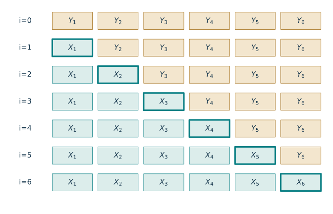
Each row changes exactly one term; the outlined cell is the term just replaced. All seven rows are shown.
We make the comparison precise using a smooth test function. Let \(\mathcal F_B\) be the functions \(\phi\in C^3(\R)\) with \(\|\phi^{(j)}\|_\infty\le B\) for \(j=0,1,2,3\), where \(\phi^{(0)}=\phi\). Such functions belong to \(C_b(\R)\); we additionally control the derivatives needed in Taylor’s formula.
Let \(X_1,X_2,\ldots\) be i.i.d., with \(\E X_1=0\), \(\E X_1^2=\sigma^2\), and \(\rho=\E|X_1|^3<\infty\). Define \(S_n=n^{-1/2}\sum_iX_i\) and \(G_\sigma\sim N(0,\sigma^2)\). Then \[\sup_{\phi\in\mathcal F_B} |\E\phi(S_n)-\E\phi(G_\sigma)| \le\frac{B}{6\sqrt n}\big(\rho+\E|G_\sigma|^3\big) \le\frac{CB\rho}{\sqrt n},\] where \(C=(1+2\sqrt{2/\pi})/6\) is a numerical constant.
Proof. Take independent \(Y_i\sim N(0,\sigma^2)\), jointly independent of all \(X_i\). Put \[S_{n,i}=\frac{X_1+\cdots+X_i+Y_{i+1}+\cdots+Y_n}{\sqrt n}, \quad i=0,\ldots,n.\] The endpoints are \(S_{n,n}=S_n\) and \(S_{n,0}\stackrel{d}{=}G_\sigma\). For \(i=0,\ldots,n-1\), let \(T_{n,i}=(X_1+\cdots+X_i+Y_{i+2}+\cdots+Y_n)/\sqrt n\). Then \(S_{n,i}=T_{n,i}+Y_{i+1}/\sqrt n\) and \(S_{n,i+1}=T_{n,i}+X_{i+1}/\sqrt n\).
Match the first two Taylor terms. For \(V=X_{i+1}\) or \(V=Y_{i+1}\), the third-order remainder bound gives
\[\begin{split} \E\phi(T_{n,i}+V/\sqrt n) ={}&\E\phi(T_{n,i}) +\frac{\E\phi'(T_{n,i})\E V}{\sqrt n}\\ &+\frac{\E\phi''(T_{n,i})\E V^2}{2n}+R_V, \qquad |R_V|\le\frac{B\E|V|^3}{6n^{3/2}}. \end{split}\]
(10)Independence of \(T_{n,i}\) and \(V\) justifies the products of expectations. The linear terms vanish and the quadratic terms agree, since both choices of \(V\) have mean zero and variance \(\sigma^2\). Hence \[|\E\phi(S_{n,i+1})-\E\phi(S_{n,i})| \le\frac{B}{6n^{3/2}}\big(\rho+\E|G_\sigma|^3\big).\] Add the replacement errors. Sum these \(n\) bounds in the telescoping identity \[\E\phi(S_n)-\E\phi(S_{n,0}) =\sum_{i=0}^{n-1}\big[\E\phi(S_{n,i+1})-\E\phi(S_{n,i})\big].\] Finally, \(\E|G_\sigma|^3=2\sqrt{2/\pi}\,\sigma^3\) and \(\sigma^3\le\rho\) by the moment inequality, giving the second bound. If \(\sigma=0\), both inputs are zero almost surely and the conclusion holds with zero error. ◻
For a fixed \(t\), both \(\cos(tx)\) and \(\sin(tx)\) lie in some \(\mathcal F_B\), for example with \(B=\max(1,|t|^3)\). Their expectation differences therefore vanish. The characteristic-function criterion gives a CLT under this argument’s stronger third-moment assumption.
Low priority — not examined: The Berry–Esseen bound
A sharper theorem measures the discrepancy between the entire CDFs, rather than between smooth test functions with a fixed derivative bound. Let \(\Phi\) denote the standard Normal CDF.
Under the preceding i.i.d. assumptions, suppose \(\sigma>0\) and \(\rho=\E|X_1|^3<\infty\). There is a universal finite constant \(C_{\rm BE}\) such that \[\sup_{a\in\R} \left|\PR\!\left(\frac{\sum_{i=1}^nX_i}{\sigma\sqrt n}\le a\right) -\Phi(a)\right| \le\frac{C_{\rm BE}\rho}{\sigma^3\sqrt n}.\] Equivalently, compare \(S_n=\sum_iX_i/\sqrt n\) with \(N(0,\sigma^2)\), using \(\Phi(a/\sigma)\) in place of \(\Phi(a)\).
Scale invariance. The standardized third absolute moment \(\rho/\sigma^3\) is unchanged when the observations are multiplied by a nonzero constant. A bound without this normalization cannot hold uniformly over scales.
CDF error. The theorem implies the CLT under its additional third-moment assumption and supplies a uniform finite-sample CDF error bound. It need not be small for a particular \(n\), and it gives no density approximation. See [1] (Section 3.4.4) for a proof.
Proof distinction. The smooth bound above is not, by itself, a proof of the same \(n^{-1/2}\) CDF rate: approximating an indicator by a narrow smooth transition makes its derivatives large. The Berry–Esseen proof needs additional control of this approximation. Exercise 12 checks the scale factors explicitly.
Detailed reference
4. Detailed reference
The table links back to each definition or statement. High and mid material are in exam scope; low material is optional enrichment. The priority in each row belongs to that item.
| Notion or result | What to remember | Tier |
|---|---|---|
| Weak convergence | CDF convergence at continuity points of the limiting CDF. | High |
| Law versus paired variables | Only distributions matter; a common probability space is unnecessary. | High |
| Probability and distribution limits | Probability convergence implies weak convergence; a constant weak limit implies concentration. | High |
| Boundedness in probability | A weakly convergent sequence is \(O_P(1)\). | High |
| Bounded continuous tests | Compare expectations of every bounded continuous function. | High |
| Characteristic function | \(\varphi_X(t)=\E e^{it^\top X}\); independent sums give products. | High |
| Cramér–Wold | Every scalar projection determines the vector limit. | High |
| Central limit theorem | Center i.i.d. sums and divide by \(\sqrt n\); assume finite second moments. | High |
| Singular covariance | Zero variance in a direction gives a constant projection. | High |
| Lévy continuity theorem | A pointwise characteristic-function limit continuous at zero is the characteristic function of a probability law. | Mid |
| Quadratic expansion | Centering cancels the linear term; a DCT remainder needs only a second moment. | Mid |
| Uniform subgaussian tails | One Gaussian-type tail bound works for the whole collection. | Low |
| Moment convergence | Uniform tail control connects unbounded moments to weak convergence. | Low |
| Pairings | Singleton indices vanish; paired indices give Gaussian leading moments. | Low |
| Lindeberg replacement | Match two moments; sum the third-order replacement errors. | Low |
| Berry–Esseen | Uniform CDF error is at most a constant times \(\rho/(\sigma^3\sqrt n)\). | Low |
| Scheffé’s theorem | Almost-everywhere convergence of normalized densities gives \(L^1\) convergence. | Low |
5. Further reading
Further reading: References and useful measure facts
For weak convergence, characteristic functions, moment determinacy and CLTs, consult [1] (Sections 3.2–3.4 and 3.10); the author’s fifth-edition book PDF is available online. Shao’s [2] (Theorem 1.9) is a standard reference for the equivalent vector criteria. The three proof approaches follow the themes of [3] (Section 2.2); Tao’s course notes on the CLT provide a companion discussion.
Some measure facts that support these arguments are worth recording:
A one-dimensional CDF has at most countably many discontinuities. These are precisely the atoms \(x\) with \(\PR(X=x)>0\). Exercise 6 gives the counting argument.
If \(B\) is a Borel subset of \(\R\) and \(m(B)<\infty\), then for any \(\varepsilon>0\) there are a compact \(K\subseteq B\) and an open \(O\supseteq B\) with \(m(B\setminus K)<\varepsilon\) and \(m(O\setminus B)<\varepsilon\). This is regularity of Lebesgue measure. For infinite-measure sets, formulate approximation locally on bounded intervals rather than subtracting \(\varepsilon\) from infinity. See Tao’s An Introduction to Measure Theory, Section 1.2 for the inner and outer regularity of Lebesgue measure.
Every open subset of \(\R\) is a countable union of disjoint open intervals, allowing unbounded endpoints. Its interval components each contain a distinct rational number, which establishes countability.
Low priority — not examined: A useful criterion for densities
For probability laws with densities \(f,g\) relative to a common measure, the total variation distance is \(\sup_A|\int_A(f-g)\,d\nu|=\tfrac12\int|f-g|\,d\nu\). It measures the largest difference in probability assigned to the same measurable event.
The following theorem also covers probability mass functions by using counting measure. Pointwise convergence of CDFs generally says nothing about pointwise convergence of their densities, so this is a separate sufficient condition.
Let \(f_n\) and \(f\) be nonnegative densities with respect to a common measure \(\nu\), with \(\int f_n\,d\nu=\int f\,d\nu=1\). If \(f_n\to f\) \(\nu\)-almost everywhere, then \[\int|f_n-f|\,d\nu\longrightarrow0.\]
In particular, probabilities of measurable sets converge uniformly: \(|\int_A(f_n-f)\,d\nu|\le\int|f_n-f|\,d\nu\). This is stronger than weak convergence and is related to total variation distance.3 Exercise 13 gives a complete proof and explains why the limiting density must still integrate to one.
Key ideas
Weak convergence concerns distributions, not a chosen pairing of observations.
The CLT needs the correct centering, normalization and assumptions.
Bounded-continuous tests, distribution functions and characteristic functions offer different checks for weak convergence.
Convergence in distribution alone does not justify convergence of moments.
Looking ahead
Lecture 11 transfers CLT approximations through transformations of an estimator. Continuous mapping, Slutsky and the delta method turn the convergence tools here into practical asymptotic calculations. Continue to Lecture 11.
6. Exercises and complete solutions13 exercises · complete solutions
Try each problem before reading its solution. The five short prompts in the main text point to Exercises 1–5 below. Further exercises supply proof details and useful extensions; each retains its own priority.
Let \(X_n=1/n\) and \(X=0\) almost surely. Write \(F_n,F\) and verify \(X_n\Rightarrow X\). Does \(F_n(0)\) converge to \(F(0)\)? Extend the argument to constants \(a_n\to a\).
Reveal solution
We have \(F_n(x)=\mathbf1\{x\ge1/n\}\) and \(F(x)=\mathbf1\{x\ge0\}\). For fixed \(x<0\), \(F_n(x)=F(x)=0\). For fixed \(x>0\), eventually \(1/n\le x\), so \(F_n(x)=F(x)=1\). These are all continuity points of \(F\), proving weak convergence. At zero, \(F_n(0)=0\) for every \(n\) but \(F(0)=1\); the definition does not require convergence at this jump. For \(a_n\to a\), any fixed \(x<a\) eventually lies below \(a_n\), and any fixed \(x>a\) eventually lies above \(a_n\). The same argument proves \(\delta_{a_n}\Rightarrow\delta_a\).
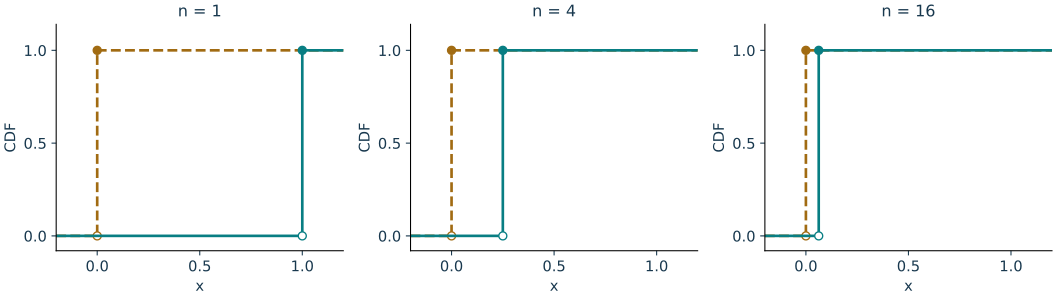
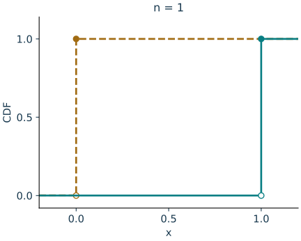
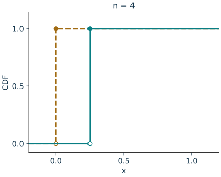
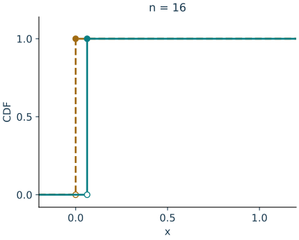
The jumps at \(1/n\) move toward zero. At zero the CDFs never agree with the limit; at every continuity point of the limit they converge.
Let \(G\sim N(0,1)\) and \(X_n=(-1)^nG\) on the same probability space. Check distributional convergence to \(G\) and decide whether convergence in probability to \(G\) holds.
Reveal solution
Symmetry gives \(X_n\stackrel{d}{=}G\) for every \(n\), so the CDFs are identical and \(X_n\Rightarrow G\). For odd \(n\), however, \(|X_n-G|=2|G|\). Thus for any \(\varepsilon>0\), \[\PR(|X_n-G|>\varepsilon)=\PR(|G|>\varepsilon/2)>0 \quad\text{for every odd $n$}.\] For even \(n\) the probability is zero. It therefore does not converge to zero, and convergence in probability to \(G\) fails.
For i.i.d. \(B_i\sim\operatorname{Bernoulli}(p)\), identify a standard Normal limit for the sample proportion when \(0<p<1\). Explain the boundary cases \(p=0,1\) and write a corresponding approximate probability for \(|\overline B_n-p|\le z\sqrt{p(1-p)/n}\), with fixed \(z>0\).
Reveal solution
Because \(B_i^2=B_i\), its mean is \(p\) and variance is \(p-p^2=p(1-p)\). The CLT gives \[T_n=\frac{\sqrt n(\overline B_n-p)}{\sqrt{p(1-p)}}\Rightarrow N(0,1).\] Both endpoints \(-z,z\) are continuity points of the Normal CDF, so \(\PR(-z\le T_n\le z)\to\Phi(z)-\Phi(-z)=2\Phi(z)-1\). For completeness, a possible atom at \(-z\) vanishes: for every \(\delta>0\), its limsup is at most \(\Phi(-z)-\Phi(-z-\delta)\), then let \(\delta\downarrow0\). This justifies the closed lower endpoint. Consequently the stated probability is approximately \(2\Phi(z)-1\) for large \(n\). If \(p=0\) or \(p=1\), every observation equals \(p\) almost surely, and the centered sample mean is exactly zero. There is a degenerate limit, and dividing by \(\sqrt{p(1-p)}\) is not defined.
Let \(X\in\R^d\) have mean \(\mu\) and finite second moments, with covariance \(\Sigma\). For fixed \(c\in\R^d\), prove that \(c^\top X\) has finite second moment, find its mean and variance, and treat \(c^\top\Sigma c=0\). Explain the vector CLT reduction.
Reveal solution
Cauchy–Schwarz gives \(|c^\top X|^2\le\|c\|^2\|X\|^2\), whose expectation is finite. Linearity gives \(\E(c^\top X)=c^\top\mu\), and \[\operatorname{Var}(c^\top X) =\E[c^\top(X-\mu)(X-\mu)^\top c]=c^\top\Sigma c.\] If this variance is zero, the nonnegative random variable \([c^\top(X-\mu)]^2\) has expectation zero, hence is zero almost surely. For a positive projected variance, the scalar CLT applies to i.i.d. \(c^\top(X_i-\mu)\). For a zero projected variance the centered sum is zero almost surely. In both cases the limit law is \(N(0,c^\top\Sigma c)\), which is the projection of \(N(0,\Sigma)\). Cramér–Wold now proves the vector statement, without an invertibility assumption on \(\Sigma\).
Low priority — not examined: Exercise 5: The fourth moment of a sum
Let \(X_i\) be i.i.d., centered, with variance one and finite fourth moment \(m_4=\E X_1^4\). For \(S_n=n^{-1/2}\sum_iX_i\), calculate \(\E S_n^4\) exactly and identify its limit. Apply the formula to signs \(X_i\in\{-1,1\}\) with equal probabilities.
Reveal solution
Only multiplicity patterns \(4\) and \(2+2\) survive: every other pattern has a singleton index, which contributes a zero mean by independence. There are \(n\) fourth-power terms. For each pair \(i<j\), there are \(4!/(2!2!)=6\) orders of the two indices. Therefore \[\E S_n^4=\frac1{n^2}\left(nm_4+6\binom n2\right) =3+\frac{m_4-3}{n}\longrightarrow3=\E G^4.\] For the signs, \(m_4=1\), so \(\E S_n^4=3-2/n\). In particular, at \(n=4\) the value is \(5/2\), also obtained directly from the five probabilities in the main example. A finite-sample fourth moment need not equal its limiting Gaussian value.
Show that a CDF has at most countably many discontinuities and justify the simultaneous choice of \(-M,M\) in part (3) of Theorem 1.
Reveal solution
The jump at \(x\) is \(F(x)-F(x-)=\PR(X=x)\), by continuity of probability from below. For each positive integer \(r\), there are at most \(r\) points with mass at least \(1/r\), since total mass is one. Every positive mass belongs to one of these finite sets; their countable union is the set of discontinuities \(D\). Given \(\varepsilon>0\), choose \(R\) so large that \(\PR(|X|\ge R)<\varepsilon/2\); the events \(\{|X|\ge R\}\) decrease to the empty set as \(R\to\infty\). Choose \(M>R\) outside the countable set \(D\cup(-D)\). Both \(-M\) and \(M\) are continuity points, and \[1-F(M)+F(-M)=\PR(X>M)+\PR(X\le-M) \le\PR(|X|\ge R)<\varepsilon/2.\] Avoiding just the discontinuities at the positive endpoint would not justify convergence at the negative endpoint as well.
Assume \(\E h(X_n)\to\E h(X)\) for every bounded continuous \(h\) on \(\R\). For a continuity point \(x\) of \(F\), use linear ramps of width \(\delta\) to prove \(F_n(x)\to F(x)\). Also verify the reverse implication for variables supported on one common finite set.
Reveal solution
Solid teal: lower ramp. Dotted gold: indicator of (−∞,0]. Dashed plum: upper ramp. The complete limiting argument is in this solution.
Let \(h_-\) equal one on \((-\infty,x-\delta]\), decrease linearly to zero on \([x-\delta,x]\), and vanish above \(x\). Let \(h_+\) equal one on \((-\infty,x]\), decrease linearly to zero on \([x,x+\delta]\), and vanish above \(x+\delta\). Both are bounded and continuous, and \(h_-\le\mathbf1_{(-\infty,x]}\le h_+\). Taking expectations and limits gives \[F(x-\delta)\le\E h_-(X)\le\liminf_nF_n(x) \le\limsup_nF_n(x)\le\E h_+(X)\le F(x+\delta).\] Let \(\delta\downarrow0\) and use continuity at \(x\). For the reverse direction on a common finite support \(\{a_1<\cdots<a_m\}\), choose \(b_0<a_1\), \(b_m>a_m\), and \(b_j\in(a_j,a_{j+1})\). All \(b_j\) are continuity points of the limit CDF, so \(\PR(X_n=a_j)=F_n(b_j)-F_n(b_{j-1})\to\PR(X=a_j)\). For any bounded continuous \(h\), sum \(h(a_j)\PR(X_n=a_j)\) over the finite set to obtain expectation convergence.
For \(\E X^2<\infty\), justify \(\psi'(t)=\E[iXe^{itX}]\) and \(\psi''(t)=-\E[X^2e^{itX}]\). Explain the use of DCT for complex-valued expressions and recover the first two derivatives at zero.
Reveal solution
The inequality \(|e^{iv}-1|\le|v|\) for real \(v\) follows by integrating \(ie^{iu}\) from \(0\) to \(v\). Consequently \[\left|\frac{e^{i(t+h)X}-e^{itX}}h\right|\le|X|.\] This bound is integrable because \(\E|X|\le(\E X^2)^{1/2}\). The difference quotient converges pointwise to \(iXe^{itX}\); apply DCT to real and imaginary parts to obtain \(\psi'(t)\). Its difference quotient is bounded by \(X^2\), so a second application gives \(\psi''(t)=-\E[X^2e^{itX}]\). DCT also shows the derivatives are continuous. At zero, \(\psi(0)=1\), \(\psi'(0)=i\E X\), and \(\psi''(0)=-\E X^2\). Centering removes the first-order term; the second-order coefficient is negative, not positive.
If \(X_n\Rightarrow X\) in \(\R^d\), prove \(AX_n+b\Rightarrow AX+b\) for a fixed matrix \(A\in\R^{k\times d}\) and a fixed vector \(b\in\R^k\). Does this require \(A\) to be invertible?
Reveal solution
For any \(h\in C_b(\R^k)\), define \(g(x)=h(Ax+b)\). The affine map is continuous, so \(g\in C_b(\R^d)\). Hence \[\E h(AX_n+b)=\E g(X_n)\longrightarrow\E g(X)=\E h(AX+b).\] The test-function criterion proves the claimed weak convergence. Neither injectivity nor invertibility is needed. This includes constant maps, centering, fixed rescaling, and projection onto a lower-dimensional space. A matrix depending on \(n\) requires an additional argument.
Low priority — not examined: Exercise 10: The boundary term in a tail moment
Derive (6) for \(Y\ge0\), \(N>0\), integer \(k\ge1\), allowing infinite expectations. Explain why deleting its first term is wrong. Apply the identity to a uniform subgaussian tail bound.
Reveal solution
For each realized value \(y\ge0\), \[y^k\mathbf1\{y>N\} =N^k\mathbf1\{y>N\}+\int_N^\infty kt^{k-1}\mathbf1\{y>t\}\,dt.\] Both sides vanish for \(y\le N\), and for \(y>N\) the integral equals \(y^k-N^k\). Tonelli gives the expectation identity. For a constant \(Y=N+\delta\), the integral alone is \((N+\delta)^k-N^k\), which can be arbitrarily small as \(\delta\downarrow0\) although the left side approaches \(N^k\). Thus no universal multiplicative constant repairs that omission for all such \(Y\). If \(\PR(Y_n>t)\le Ce^{-ct^2}\) uniformly in \(n\), the missing boundary term is at most \(CN^ke^{-cN^2}\to0\). The integral remainder is at most \(C\int_N^\infty kt^{k-1}e^{-ct^2}\,dt\to0\), as the integrand is integrable. Together these prove uniform decay of the tail moments.
Low priority — not examined: Exercise 11: A tail bound for bounded summands
Suppose the independent variables \(X_i\) have mean zero and \(|X_i|\le M\), where \(M>0\). Show that \(S_n=n^{-1/2}\sum_{i=1}^nX_i\) satisfies \(\PR(|S_n|\ge t)\le2e^{-t^2/(2M^2)}\) for \(t>0\), uniformly in \(n\).
Reveal solution
Convexity on \([-M,M]\) yields, for real \(s\), \[e^{sx}\le\frac{M+x}{2M}e^{sM}+\frac{M-x}{2M}e^{-sM}.\] Take expectations and use \(\E X_i=0\) to get \(\E e^{sX_i}\le\cosh(sM)\le e^{s^2M^2/2}\). The last inequality follows by comparing power series, since \((2j)!\ge2^jj!\). Independence therefore gives \(\E e^{sS_n}\le e^{s^2M^2/2}\). For \(s>0\), Markov’s inequality gives \(\PR(S_n\ge t)\le e^{-st+s^2M^2/2}\). Choose \(s=t/M^2\) to obtain \(e^{-t^2/(2M^2)}\). Apply the same argument to \(-S_n\) and add the two bounds. These constants do not depend on \(n\), proving the uniform subgaussian property needed in the moment proof.
Low priority — not examined: Exercise 12: Checking the scale in Normal approximation
For a centered variable with variance \(\sigma^2>0\) and \(\rho=\E|X|^3<\infty\), prove \(\rho\ge\sigma^3\) and calculate \(\E|G_\sigma|^3\) for \(G_\sigma\sim N(0,\sigma^2)\). Show why Berry–Esseen uses \(\rho/\sigma^3\), and specialize the smooth and CDF bounds to \(X=\pm2\) with equal probabilities.
Reveal solution
Apply Jensen to \(u^{3/2}\) and \(U=|X|^2\): \(\rho=\E U^{3/2}\ge(\E U)^{3/2}=\sigma^3\). For \(G\sim N(0,1)\), symmetry and the change of variable \(u=x^2/2\) give \[\E|G|^3=\frac2{\sqrt{2\pi}}\int_0^\infty x^3e^{-x^2/2}\,dx =\frac4{\sqrt{2\pi}}\int_0^\infty ue^{-u}\,du =2\sqrt{2/\pi}.\] Thus \(\E|G_\sigma|^3=2\sqrt{2/\pi}\,\sigma^3\). The standardized input \(X/\sigma\) has variance one and third absolute moment \(\rho/\sigma^3\). Replacing \(X\) by \(aX\), \(a\ne0\), multiplies both \(\rho\) and \(\sigma^3\) by \(|a|^3\), leaving their ratio unchanged. For \(X=\pm2\), \(\sigma^2=4\) and \(\rho=8\). The smooth bound compares \(S_n\) with \(N(0,4)\) and is at most \(8(1+2\sqrt{2/\pi})B/(6\sqrt n)\). The CDF bound compares \(S_n/2\) with \(N(0,1)\) and is at most \(C_{\rm BE}/\sqrt n\), or equivalently compares \(\PR(S_n\le a)\) with \(\Phi(a/2)\) at that same rate.
Low priority — not examined: Exercise 13: Scheffé’s theorem and loss of mass
Prove Theorem 8 using \(\min(f_n,f)\). Explain the necessity of \(\int f\,d\nu=1\) by considering \(f_n(x)=\mathbf1_{[n,n+1]}(x)\) on \(\R\). Verify the factor \(1/2\) in total variation distance for two densities.
Reveal solution
We have \(\min(f_n,f)\to f\) almost everywhere and \(0\le\min(f_n,f)\le f\), with \(f\) integrable. DCT gives \(\int\min(f_n,f)\,d\nu\to1\). Since \(|a-b|=a+b-2\min(a,b)\) for nonnegative \(a,b\), \[\int|f_n-f|\,d\nu=2-2\int\min(f_n,f)\,d\nu\longrightarrow0.\] For the shifting interval densities, \(f_n(x)\to0\) at every fixed \(x\), but \(\int f_n\,dx=1\). The zero limit is not a probability density, and \(\int|f_n-0|\,dx=1\); probability mass escapes to infinity. Finally set \(h=f-g\). Because \(\int h=0\), \(\int h^+=\int h^-=\tfrac12\int|h|\). For every measurable \(A\), \(-\int h^-\le\int_Ah\le\int h^+\), with the upper endpoint attained at \(A=\{h>0\}\). This proves \(\sup_A|\int_A(f-g)|=\tfrac12\int|f-g|\).
References
Terminology notes
A Fourier transform describes a function or measure by its responses to oscillations at different frequencies. For a probability measure \(\mu\), \(\int e^{it^\top x}\,d\mu(x)\) is its characteristic function, with a choice of sign convention. It is the transform of the probability measure, rather than of the CDF viewed as an ordinary integrable function.↩︎
Standard Brownian motion is a continuous random path \(B(t)\), \(t\ge0\), starting at zero, with independent increments and \(B(t)-B(s)\sim N(0,t-s)\) for \(t>s\). It models accumulated random fluctuations over time. Process-level convergence to such paths requires more than the scalar CLT stated here.↩︎
Total variation distance · Low — not examined
For probability laws with densities \(f,g\) relative to a common measure, the total variation distance is \(\sup_A|\int_A(f-g)\,d\nu|=\tfrac12\int|f-g|\,d\nu\). It measures the largest difference in probability assigned to the same measurable event.↩︎
What changed
October 19, 2026: Corrected notation, wording and cross-references after the course-wide errata review; refreshed the linked HTML and PDF editions.
October 14, 2026. Added issue-reporting links to the webpage and PDF. The mathematics and priority assignments are unchanged in this update.
Comments
Discuss an idea or ask a public question. Include a section or exercise number when relevant. For errors in the notes or website, Report an issue.
Public comments use Disqus. Enable JavaScript to load them.
Email the instructor for a private question or if comments are unavailable.