STAT 709 · Lecture 9 · Convergence, laws of large numbers, and consistency

These notes support STAT 709 at the University of Wisconsin–Madison. Use them alongside the cited textbooks; corrections and questions are welcome.

High priorityAsymptotic properties of estimators

Overview.

Asymptotic properties of estimators. Lecture 8 introduced methods for constructing estimators. This lecture studies conditions under which their estimation errors vanish as the sample size increases. The main tools are convergence in probability, stochastic orders, and laws of large numbers. Laws of large numbers establish convergence of empirical averages to population expectations; continuity and uniform convergence then yield consistency results for moment estimators and minimizers of sample objectives. We distinguish convergence at a fixed argument from uniform convergence over a family of arguments.
Organization of the lecture. We first develop the weak law and use it to justify moment estimators. The optional strong-law and uniform-law sections develop almost-sure and uniform convergence. The final applications concern regression and maximum likelihood, including a uniform-endpoint estimator with a rate faster than $n^{-1/2}$ $n^{-1/2}$ .

Mid priorityNotation and conventions

Notation conventions. We write $\E X$ $\mathbb{E}X$ or $\E[X]$ $\mathbb{E}[X]$ for expectation and $\PR(A)$ $\mathbb{P}(A)$ for the probability of an event. Uppercase letters usually denote random variables and lowercase letters their possible values; $\R$ $\mathbb{R}$ denotes the real numbers and $\mathbf 1_A$ $\mathbf 1_A$ the indicator of $A$ $A$ . This follows the probability notation used by Shao and many statistics texts. Machine-learning papers often make different choices, such as bold vectors and a distinction between random variables and their realizations by font. The Deep Learning notation guide is a useful comparison. Check the notation conventions when comparing formulas.
Fixed-dimensional setting. Throughout, limits are as $n\to\infty$ $n\to\infty$ , and vectors have a fixed finite dimension unless we explicitly say otherwise.

This begins Part III. The part overview connects these lectures and includes a final self-check.

Recap from earlier lecturesFrom Lectures 1, 3, 4 and 8: estimator recipes and limits · 1 min

Reminder only: this block introduces no new exam requirements.

Moment and likelihood estimators. Sample moments are matched to model moments; likelihood is maximized over the parameter. Used in Section 7.
Population likelihood. The KL inequality identifies the truth as a population likelihood maximizer. Used in optional Section 7.3.
Markov and Chebyshev. Moment bounds turn into bounds on error probabilities. Used in Section 4.1.
Dominated convergence. An integrable bound permits the limit to pass through an integral. Used in Section 4.2.
Compactness. A continuous function attains its extrema on a nonempty compact set. Used in Section 7.2.

Learning goals

Distinguish probability limits, almost-sure limits, and stochastic rates.
Prove a weak law by variance control and apply the integrable weak law.
Check the assumptions behind consistency of moments and minimizers.
Explain why pointwise convergence alone does not control optimization.

1. Exact inference and the asymptotic approach

Mid priorityMotivation for asymptotic analysis

Finite-sample error. At a fixed sample size, we study the error of an estimator relative to its population target. Exact calculations of bias or variance are available in some models, but can be difficult in others.
Asymptotic analysis. An asymptotic approach studies an estimator as the sample size increases. A basic question is whether its error becomes small with high probability.
Sample-mean convergence. The sample mean is the starting example. A law of large numbers gives conditions under which this average converges to the population mean, justifying estimation by empirical averages.

Quick Explanation

Empirical process

Edgeworth expansion

Instructor’s NoteAsymptotic approximation and model complexity

Convergence and fluctuations. Think of increasing the sample size as turning up the resolution of a picture. First we ask whether the estimate settles near the right target; then we can zoom in on the remaining fluctuations. The LLN addresses the first question; the central limit theorem (CLT) often answers the second. Exact calculations, such as the usual $t$ $t$ distribution under a Normal model, give another way to study sampling error.
Dimension and model complexity. The picture also changes if we add more unknown parameters as we collect more observations. The regression examples in Lecture 7 illustrate this balance between sample size and model complexity. Classical asymptotics often holds dimension fixed; random matrix theory and empirical-process methods help study richer settings.¹ The relative growth of data and dimension matters.
Methods for uncertainty assessment. Other methods address uncertainty at the observed sample size: finite-sample corrections and Edgeworth expansions refine an approximation,² the bootstrap creates new samples by drawing with replacement from the observed data, and Bayesian modeling brings domain knowledge into the analysis. Subsampling is a related but different resampling idea. Think of these as different tools for understanding uncertainty. For now, our task is simply to understand why averages stabilize.

2. Convergence in probability

2.1. Modes of stochastic convergence

High priorityAlmost-sure convergence and convergence in probability

Let $X,X_1,X_2,\ldots$ $X,X_1,X_2,\ldots$ be random vectors in $\R^k$ $\mathbb{R}^k$ on a common probability space, with Euclidean norm $\|\cdot\|$ $\|\cdot\|$ .

Definition 1

The sequence converges almost surely to $X$ $X$ , written $X_n\to X$ $X_n\to X$ a.s., if \[\PR\{\omega:\|X_n(\omega)-X(\omega)\|\to0\}=1.\] $\mathbb{P}\{\omega:\|X_n(\omega)-X(\omega)\|\to0\}=1.$

Definition 2

The sequence converges in probability to $X$ $X$ , written $X_n\xrightarrow{P}X$ $X_n\overset{P}{\longrightarrow}X$ , if for every $\varepsilon>0$ $\varepsilon>0$ , \[\PR(\|X_n-X\|>\varepsilon)\longrightarrow0.\] $\mathbb{P}(\|X_n-X\|>\varepsilon)\longrightarrow0.$

Convergence to a constant in probability can also be defined when each $X_n$ $X_n$ lives on its own probability space. Almost-sure convergence concerns entire sample paths and therefore requires a common probability space.

Instructor’s NoteMarginal probabilities and sample-path behavior

Intuitively, convergence in probability looks at one photograph for each sample size: what fraction of experiments are still far from the target? Almost-sure convergence watches the whole movie of one experiment as more observations arrive. Along almost every movie, the errors eventually stay inside every fixed tolerance. The random variables have to “work together” across time for this second statement; small error probabilities in separate photographs do not tell the whole story.

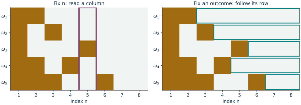
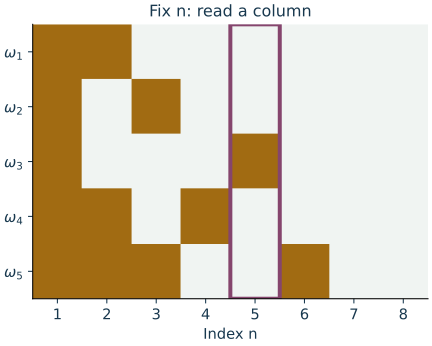
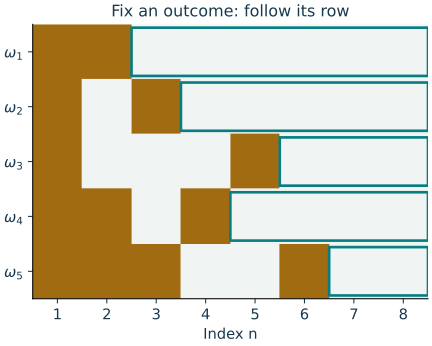
Gold cells mark errors exceeding a fixed tolerance. A column compares outcomes at one n; each row follows one outcome through time. The finite schematic illustrates the quantifiers, not a proof of convergence.

Columns compare outcomes at a fixed index; rows follow one outcome through time. Gold cells mark errors above a fixed tolerance. This finite schematic illustrates the quantifiers, not a limit theorem.

High priorityAlmost-sure convergence implies convergence in probability

Fix $\varepsilon>0$ $\varepsilon>0$ and put \[A_{n,\varepsilon}=\{\|X_n-X\|\le\varepsilon\},\qquad B_{N,\varepsilon}=\bigcap_{n\ge N}A_{n,\varepsilon}.\] $A_{n,\varepsilon}=\{\|X_n-X\|\le\varepsilon\},\qquad B_{N,\varepsilon}=\bigcap_{n\ge N}A_{n,\varepsilon}.$ If $X_n\to X$ $X_n\to X$ a.s., then $B_{N,\varepsilon}$ $B_{N,\varepsilon}$ increases with $N$ $N$ and $\PR(\bigcup_N B_{N,\varepsilon})=1$ $\mathbb{P}(\bigcup_N B_{N,\varepsilon})=1$ . Continuity of probability from below and $B_{N,\varepsilon}\subset A_{N,\varepsilon}$ $B_{N,\varepsilon}\subset A_{N,\varepsilon}$ give

\[\PR(B_{N,\varepsilon})\to1 \quad\Longrightarrow\quad \PR(A_{N,\varepsilon})\to1.\] $\mathbb{P}(B_{N,\varepsilon})\to1 \quad\Longrightarrow\quad \mathbb{P}(A_{N,\varepsilon})\to1.$

(1)

This proves convergence in probability. More explicitly, the pathwise convergence event can be written using the countable tolerances $1/m$ $1/m$ as $\bigcap_{m\ge1}\bigcup_N B_{N,1/m}$ $\bigcap_{m\ge1}\bigcup_N B_{N,1/m}$ ; this also explains its measurability. The converse implication between the two modes is false: see Exercise 7 and its complete counterexample.

High priorityFirst Borel–Cantelli lemma and almost-sure convergence

Proposition 1First Borel–Cantelli lemma

If events $E_n$ $E_n$ satisfy $\sum_n\PR(E_n)<\infty$ $\sum_n\mathbb{P}(E_n)<\infty$ , then with probability one only finitely many $E_n$ $E_n$ occur. No independence is needed.

Indeed, \[\PR\Big(\bigcup_{n\ge N}E_n\Big)\le\sum_{n\ge N}\PR(E_n)\to0.\] $\mathbb{P}\Big(\bigcup_{n\ge N}E_n\Big)\le\sum_{n\ge N}\mathbb{P}(E_n)\to0.$ The events on the left decrease to the event that infinitely many $E_n$ $E_n$ occur, so continuity from above proves the claim. In particular, if $\sum_n\PR(\|X_n-X\|>\varepsilon)<\infty$ $\sum_n\mathbb{P}(\|X_n-X\|>\varepsilon)<\infty$ for every $\varepsilon>0$ $\varepsilon>0$ , apply the proposition at $\varepsilon=1/m$ $\varepsilon=1/m$ and intersect the resulting probability-one events to obtain $X_n\to X$ $X_n\to X$ a.s. Exercise 8 gives a second proof by counting errors and interchanging a nonnegative sum with expectation.

2.2. Stochastic orders

High priorityStochastic orders and Gaussian examples

For deterministic positive $a_n$ $a_n$ , the familiar notation $x_n=o(a_n)$ $x_n=o(a_n)$ means $x_n/a_n\to0$ $x_n/a_n\to0$ , while $x_n=O(a_n)$ $x_n=O(a_n)$ means that $|x_n|/a_n$ $|x_n|/a_n$ is eventually bounded. Random errors need probabilistic versions.

Definition 3

For deterministic $a_n>0$ $a_n>0$ , write $X_n=o_P(a_n)$ $X_n=o_P(a_n)$ if $\|X_n\|/a_n\xrightarrow{P}0$ $\|X_n\|/a_n\overset{P}{\longrightarrow}0$ . Write $X_n=O_P(a_n)$ $X_n=O_P(a_n)$ , or say that $X_n/a_n$ $X_n/a_n$ is bounded in probability, if for every $\eta>0$ $\eta>0$ there are finite $M$ $M$ and $N$ $N$ such that \[\sup_{n\ge N}\PR(\|X_n\|>Ma_n)<\eta.\] $\sup_{n\ge N}\mathbb{P}(\|X_n\|>Ma_n)<\eta.$

Convergence and stochastic boundedness. Thus $o_P(1)$ $o_P(1)$ means convergence in probability to zero; $O_P(1)$ $O_P(1)$ permits persistent random variation.
Uniform bounds over all indices. For finite-valued $X_n$ $X_n$ and positive $a_n$ $a_n$ , one may equivalently take the supremum over all $n\ge1$ $n\ge1$ : enlarge $M$ $M$ to control the finitely many omitted indices. The distinction between a small random error and an error that stays on a fixed scale is essential.

Example 1

For $X_n\sim N(0,\sigma_n^2)$ $X_n\sim N(0,\sigma_n^2)$ , bounded $\sigma_n$ $\sigma_n$ gives $O_P(1)$ $O_P(1)$ , even if $X_n$ $X_n$ does not converge to zero. If $\sigma_n\to0$ $\sigma_n\to0$ , then $X_n=o_P(1)$ $X_n=o_P(1)$ ; if $\sigma_n\to\infty$ $\sigma_n\to\infty$ , it is not $O_P(1)$ $O_P(1)$ . No particular dependence between the $X_n$ $X_n$ is needed for these claims.

Mid priorityRandom scaling and the product rule for stochastic orders

Random normalizations. Random-scale notation can also be useful. If $\PR(|Y_n|>0)=1$ $\mathbb{P}(|Y_n|>0)=1$ for every $n$ $n$ , define $X_n=o_P(Y_n)$ $X_n=o_P(Y_n)$ and $O_P(Y_n)$ $O_P(Y_n)$ by applying the preceding definitions to $\|X_n\|/|Y_n|$ $\|X_n\|/|Y_n|$ . If a denominator can be zero, first specify how that event is handled; an undefined ratio is not a stochastic-order statement.
Inclusion and product rules. For deterministic positive scales, $o_P(a_n)$ $o_P(a_n)$ implies $O_P(a_n)$ $O_P(a_n)$ . Also, for real random variables, \[U_n=o_P(a_n),\quad V_n=O_P(b_n) \quad\Longrightarrow\quad U_nV_n=o_P(a_nb_n).\] $U_n=o_P(a_n),\quad V_n=O_P(b_n) \quad\Longrightarrow\quad U_nV_n=o_P(a_nb_n).$
Dependence between the factors. There is no independence assumption. A useful proof splits according to whether $|V_n|/b_n$ $|V_n|/b_n$ exceeds a large constant; Exercise 6 gives the complete argument.

3. Consistency of estimators

High priorityConsistency and rates of convergence

Quick Recall

Stochastic orders

Let $X^{(n)}=(X_1,\ldots,X_n)$ $X^{(n)}=(X_1,\ldots,X_n)$ be the data, with a distribution determined by $P$ $P$ in a model $\mathcal P$ $\mathcal P$ , and let $\nu(P)\in\R^k$ $\nu(P)\in\mathbb{R}^k$ be the estimand. An estimator $T_n=T_n(X^{(n)})$ $T_n=T_n(X^{(n)})$ is a measurable function of the observations.

Definition 4

The sequence $T_n$ $T_n$ is consistent for $\nu$ $\nu$ if, for every fixed $P\in\mathcal P$ $P\in\mathcal P$ , $T_n\xrightarrow{P}\nu(P)$ $T_n\overset{P}{\longrightarrow}\nu(P)$ under $P$ $P$ . For deterministic $a_n>0$ $a_n>0$ with $a_n\to\infty$ $a_n\to\infty$ , it is $a_n$ $a_n$ -consistent if $a_n\{T_n-\nu(P)\}=O_P(1)$ $a_n\{T_n-\nu(P)\}=O_P(1)$ for every fixed $P$ $P$ . It is strongly consistent if $T_n\to\nu(P)$ $T_n\to\nu(P)$ a.s. under each $P$ $P$ , on a common space carrying the data sequence.

Pointwise consistency. Recall the earlier definition of stochastic orders when interpreting the rate. The quantifier “for every fixed $P$ $P$ ” describes pointwise consistency; it does not assert that the worst error probability over all $P\in\mathcal P$ $P\in\mathcal P$ tends to zero.
Stochastic convergence rates. A stochastic rate is an upper bound on the error scale, not a claim that this is the best possible rate.
Square-root convergence rates. For example, $\sqrt n$ $\sqrt n$ -consistency says the error is $O_P(n^{-1/2})$ $O_P(n^{-1/2})$ . It neither says that the error is eventually bounded by $n^{-1/2}$ $n^{-1/2}$ on every sample path nor supplies a limiting distribution.

Instructor’s NoteInterpretation of consistency and convergence rates

Imagine collecting larger data sets and applying the same estimation procedure each time. Consistency asks whether the estimates concentrate near the population target. A convergence rate describes the scale of the remaining error. Rescaling the errors lets us compare their magnitudes at different sample sizes. This thought experiment helps us understand a procedure even when only one data set is available.

Mid priorityAsymptotic and finite-sample guarantees

Finite-sample guarantees. A finite-sample guarantee might say that, for every $n\ge3$ $n\ge3$ , an error bound holds with probability at least $1-2/n$ $1-2/n$ . Such a statement can imply consistency when its error bound tends to zero, and it also tells us how the guarantee depends on the actual $n$ $n$ .
Asymptotic guarantees. Asymptotic statements instead emphasize the eventual behavior, often with simpler formulas.

Instructor’s NoteAsymptotic limits and sample-size requirements

Informally, many statistics arguments ask, “What happens as data become abundant?” Many theoretical computer-science arguments ask, “How many samples are enough for this accuracy and failure probability?” It is useful to understand both perspectives. A limit describes the behavior as sample size increases; a finite-sample bound quantifies the sample size needed for a specified accuracy.

Consistency alone does not compare finite-sample risk. The shrinkage and bias–variance examples in Lecture 7 already show why we also care about the magnitude of error at the sample size we have.

4. Laws of large numbers

4.1. Weak law under bounded variances

High priorityWeak law for uncorrelated observations

Theorem 1

Suppose $X_1,X_2,\ldots$ $X_1,X_2,\ldots$ are pairwise uncorrelated real random variables, $\E X_i=\mu$ $\mathbb{E}X_i=\mu$ , and $\Var(X_i)\le C<\infty$ $\mathrm{Var}(X_i)\le C<\infty$ . Then $\bar X_n=n^{-1}\sum_{i=1}^nX_i\xrightarrow{P}\mu$ $\bar X_n=n^{-1}\sum_{i=1}^nX_i\overset{P}{\longrightarrow}\mu$ .

Proof. Uncorrelatedness eliminates the cross-covariances, so

\[\E(\bar X_n-\mu)^2=\Var(\bar X_n) =\frac1{n^2}\sum_{i=1}^n\Var(X_i)\le\frac Cn.\] $\mathbb{E}(\bar X_n-\mu)^2=\mathrm{Var}(\bar X_n) =\frac1{n^2}\sum_{i=1}^n\mathrm{Var}(X_i)\le\frac Cn.$

(2)

The right side tends to zero: this is $L^2$ $L^2$ convergence. Chebyshev’s inequality below gives $\PR(|\bar X_n-\mu|>\varepsilon)\le C/(n\varepsilon^2)\to0$ $\mathbb{P}(|\bar X_n-\mu|>\varepsilon)\le C/(n\varepsilon^2)\to0$ . ◻

Theorem 2Chebyshev’s inequality

If $\E Y^2<\infty$ $\mathbb{E}Y^2<\infty$ and $\varepsilon>0$ $\varepsilon>0$ , then \[\PR(|Y-\E Y|>\varepsilon) \le\frac{\E[(Y-\E Y)^2]}{\varepsilon^2} =\frac{\Var(Y)}{\varepsilon^2}.\] $\mathbb{P}(|Y-\mathbb{E}Y|>\varepsilon) \le\frac{\mathbb{E}[(Y-\mathbb{E}Y)^2]}{\varepsilon^2} =\frac{\mathrm{Var}(Y)}{\varepsilon^2}.$

It follows immediately from Markov’s inequality applied to $(Y-\E Y)^2$ $(Y-\mathbb{E}Y)^2$ . In particular, $\E|Y_n-Y|^2\to0$ $\mathbb{E}|Y_n-Y|^2\to0$ implies $Y_n\xrightarrow{P}Y$ $Y_n\overset{P}{\longrightarrow}Y$ by the same argument, without requiring the errors to have mean zero. For i.i.d. variables with variance $\sigma^2<\infty$ $\sigma^2<\infty$ , the bound also gives $\sqrt n(\bar X_n-\mu)=O_P(1)$ $\sqrt n(\bar X_n-\mu)=O_P(1)$ .

Mid priorityMoment inequalities and integrability conditions

Moment inequalities. On a probability space, if $0<p<q$ $0<p<q$ and $R=\|X\|$ $R=\|X\|$ for a fixed norm, then \[(\E R^p)^{1/p}\le(\E R^q)^{1/q}.\] $(\mathbb{E}R^p)^{1/p}\le(\mathbb{E}R^q)^{1/q}.$ When $\E R^q<\infty$ $\mathbb{E}R^q<\infty$ , Jensen’s inequality for the concave function $u\mapsto u^{p/q}$ $u\mapsto u^{p/q}$ proves this; if the right side is infinite, the inequality holds in the extended real sense. Thus a finite higher moment implies a finite lower moment. This compares moments of the same nonnegative variable, not different coordinate norms of a vector.
Square-integrable random variables. Another useful viewpoint comes from functional analysis: square-integrable random variables belong to $L^2(\Omega)$ $L^2(\Omega)$ , with $\|Y\|_{L^2}=(\E|Y|^2)^{1/2}$ $\|Y\|_{L^2}=(\mathbb{E}|Y|^2)^{1/2}$ (identifying variables equal a.s.). Thus (2) states $\|\bar X_n-\mu\|_{L^2}\to0$ $\|\bar X_n-\mu\|_{L^2}\to0$ . For bounded $R$ $R$ , the moment comparison also has the endpoint $(\E R^p)^{1/p}\le\mathop{\rm ess\,sup}R$ $(\mathbb{E}R^p)^{1/p}\le\mathop{\mathrm{ess\,sup}}R$ , the smallest a.s. upper bound.

A finite lower moment does not imply a finite higher one. A Pareto variable with tail $\PR(X>t)=t^{-\alpha}$ $\mathbb{P}(X>t)=t^{-\alpha}$ for $t\ge1$ $t\ge1$ and $1<\alpha<2$ $1<\alpha<2$ has finite mean and infinite second moment; Exercise 9 contains the calculation. The variance-based proof does not apply to this example. A weak law remains available under a finite first absolute moment.

A finite mean, an infinite second moment

As the cutoff grows, which accumulated moment approaches a finite limit?

Cutoff R = 10ᵘ: 10
First capped moment A₁(R): 2.368
Second capped moment A₂(R): 9.649
Population mean α/(α − 1): 3

The shaded regions show the full areas from 0 to R, including the contribution on [0, 1]. Readouts are rounded; the formulas in the explanation are exact.

Shape α

Logarithmic cutoff u = log₁₀ R

Cutoff R = 10ᵘ: 10
First capped moment A₁(R): 2.368
Second capped moment A₂(R): 9.649
Population mean α/(α − 1): 3

The shaded regions show the full areas from 0 to R, including the contribution on [0, 1]. Readouts are rounded; the formulas in the explanation are exact.

The figure uses exact tail integrals, not samples. How to read the figure and static values · Complete moment calculation

Reading the moment areas

Picture: accumulating moment areas.

For this Pareto example, which accumulated moment approaches a finite limit as the cutoff increases, and which grows without bound? The tail-integral identity gives, for $R\ge1$ $R\ge1$ , \[A_1(R)=\int_0^R\PR(X>t)\,dt=\E\min(X,R),\qquad A_2(R)=\int_0^R2t\PR(X>t)\,dt=\E[\min(X,R)^2].\] $A_1(R)=\int_0^R\mathbb{P}(X>t)\,dt=\mathbb{E}\min(X,R),\qquad A_2(R)=\int_0^R2t\mathbb{P}(X>t)\,dt=\mathbb{E}[\min(X,R)^2].$ Both integrals contribute area $1$ $1$ on $[0,1]$ $[0,1]$ . On $[1,R]$ $[1,R]$ , integrate $t^{-\alpha}$ $t^{-\alpha}$ and $2t^{1-\alpha}$ $2t^{1-\alpha}$ to obtain \[A_1(R)=1+\frac{1-R^{1-\alpha}}{\alpha-1},\qquad A_2(R)=1+\frac{2(R^{2-\alpha}-1)}{2-\alpha}.\] $A_1(R)=1+\frac{1-R^{1-\alpha}}{\alpha-1},\qquad A_2(R)=1+\frac{2(R^{2-\alpha}-1)}{2-\alpha}.$ These are capped moments; capping at $R$ $R$ differs from setting observations above $R$ $R$ to zero in the truncation argument below. For $\alpha=3/2$ $\alpha=3/2$ , the following values give a static comparison.

Cutoff $R$ $R$	$A_1(R)$ $A_1(R)$	$A_2(R)$ $A_2(R)$
$1$ $1$	$1$ $1$	$1$ $1$
$10$ $10$	$3-2/\sqrt{10}\approx2.368$ $3-2/\sqrt{10}\approx2.368$	$4\sqrt{10}-3\approx9.649$ $4\sqrt{10}-3\approx9.649$
$100$ $100$	$2.8$ $2.8$	$37$ $37$

The first area approaches $\alpha/(\alpha-1)$ $\alpha/(\alpha-1)$ ; the second grows without bound. A finite picture shows only finite areas. The complete infinite-moment calculation is in Exercise 9 and its solution.

4.2. Truncation and a finite first moment

Mid priorityWeak law with truncated centering

Theorem 3

Let $X_1,X_2,\ldots$ $X_1,X_2,\ldots$ be i.i.d. real random variables. Assume $n\PR(|X_1|>n)\to0$ $n\mathbb{P}(|X_1|>n)\to0$ and define \[a_n=\E[X_1\mathbf 1_{\{|X_1|\le n\}}].\] $a_n=\mathbb{E}[X_1\mathbf 1_{\{|X_1|\le n\}}].$ Then

\[\frac1n\sum_{j=1}^nX_j-a_n\xrightarrow{P}0.\] $\frac1n\sum_{j=1}^nX_j-a_n\overset{P}{\longrightarrow}0.$

(3)

Low priority — not examined: Proof by truncation and variance control

Quick Recall

Chebyshev’s inequality

Proof (optional). Put $Y_{n,j}=X_j\mathbf 1_{\{|X_j|\le n\}}$ $Y_{n,j}=X_j\mathbf 1_{\{|X_j|\le n\}}$ , $S_n=n^{-1}\sum_{j=1}^nX_j$ $S_n=n^{-1}\sum_{j=1}^nX_j$ , and $T_n=n^{-1}\sum_{j=1}^nY_{n,j}$ $T_n=n^{-1}\sum_{j=1}^nY_{n,j}$ . Within each row $n$ $n$ , the $Y_{n,j}$ $Y_{n,j}$ are i.i.d. and $\E T_n=a_n$ $\mathbb{E}T_n=a_n$ . The rows need not be independent. By the union bound,

\[\PR(S_n\ne T_n)\le\PR\Big(\bigcup_{j=1}^n\{|X_j|>n\}\Big) \le n\PR(|X_1|>n)\to0.\] $\mathbb{P}(S_n\ne T_n)\le\mathbb{P}\Big(\bigcup_{j=1}^n\{|X_j|>n\}\Big) \le n\mathbb{P}(|X_1|>n)\to0.$

(4)

The cutoff includes observations equal to $n$ $n$ in absolute value; the discarded event is therefore $|X_j|>n$ $|X_j|>n$ , also for distributions with atoms. For $Z=|X_1|$ $Z=|X_1|$ , the nonnegative tail-integral identity from Lecture 4 gives \[\E Y_{n,1}^2\le\E[\min(Z,n)^2] =2\int_0^n t\PR(Z>t)\,dt.\] $\mathbb{E}Y_{n,1}^2\le\mathbb{E}[\min(Z,n)^2] =2\int_0^n t\mathbb{P}(Z>t)\,dt.$ The integer tail condition implies $t\PR(Z>t)\to0$ $t\mathbb{P}(Z>t)\to0$ for real $t$ $t$ : with $m=\lfloor t\rfloor\ge1$ $m=\lfloor t\rfloor\ge1$ , it is at most $(m+1)\PR(Z>m)$ $(m+1)\mathbb{P}(Z>m)$ . If $g(t)=t\PR(Z>t)$ $g(t)=t\mathbb{P}(Z>t)$ , then for any $\delta>0$ $\delta>0$ choose $R$ $R$ so that $g(t)\le\delta$ $g(t)\le\delta$ for $t\ge R$ $t\ge R$ . Since $g(t)\le t$ $g(t)\le t$ , \[\frac1n\int_0^n g(t)\,dt \le\frac1n\int_0^R g(t)\,dt+\delta\qquad(n\ge R).\] $\frac1n\int_0^n g(t)\,dt \le\frac1n\int_0^R g(t)\,dt+\delta\qquad(n\ge R).$ The limsup is at most $\delta$ $\delta$ . As $\delta$ $\delta$ is arbitrary, the integral average tends to zero. The earlier Chebyshev inequality now yields \[\PR(|T_n-a_n|>\varepsilon) \le\frac{\Var(Y_{n,1})}{n\varepsilon^2} \le\frac{2}{n\varepsilon^2}\int_0^n g(t)\,dt\to0.\] $\mathbb{P}(|T_n-a_n|>\varepsilon) \le\frac{\mathrm{Var}(Y_{n,1})}{n\varepsilon^2} \le\frac{2}{n\varepsilon^2}\int_0^n g(t)\,dt\to0.$ Finally $\PR(|S_n-a_n|>\varepsilon)$ $\mathbb{P}(|S_n-a_n|>\varepsilon)$ is at most the last probability plus $\PR(S_n\ne T_n)$ $\mathbb{P}(S_n\ne T_n)$ , proving the result. ◻

High prioritySample mean converges to population mean

Theorem 4Weak LLN for integrable i.i.d. observations

If the $X_i$ $X_i$ are i.i.d. and $\E|X_1|<\infty$ $\mathbb{E}|X_1|<\infty$ , then $\bar X_n\xrightarrow{P}\mu=\E X_1$ $\bar X_n\overset{P}{\longrightarrow}\mu=\mathbb{E}X_1$ .

Instructor’s NoteVariance reduction and truncation

Think of averaging as a noise-canceling operation: centered cross terms cancel in expectation, so the average has much less fluctuation than an individual observation. Rare large observations can dominate the sample mean. Truncation temporarily sets those observations aside. We choose the cutoff so that discarding any observation is unlikely, while the variance of the average of $n$ $n$ truncated observations tends to zero. We then recover the original average because it agrees with the truncated average with high probability.

Mid priorityWeak law for random vectors

If $X_i\in\R^k$ $X_i\in\mathbb{R}^k$ are i.i.d. with $\E\|X_1\|<\infty$ $\mathbb{E}\|X_1\|<\infty$ , each coordinate is integrable. Coordinatewise weak LLNs and the union bound give \[\PR(\|\bar X_n-\E X_1\|>\varepsilon) \le\sum_{j=1}^k \PR\bigl(|\bar X_{n,j}-\E X_{1,j}|>\varepsilon/\sqrt{k}\bigr)\to0.\] $\mathbb{P}(\|\bar X_n-\mathbb{E}X_1\|>\varepsilon) \le\sum_{j=1}^k \mathbb{P}\left(|\bar X_{n,j}-\mathbb{E}X_{1,j}|>\varepsilon/\sqrt{k}\right)\to0.$ Here $k$ $k$ is fixed. Increasing $k$ $k$ changes both the number of error events and their tolerances, so this proof does not by itself give a high-dimensional law.

5. Strong laws and tail events (optional)

Low priority — not examined: Tail events and Kolmogorov’s zero–one law

For real $X_1,X_2,\ldots$ $X_1,X_2,\ldots$ , put \[\mathcal F'_m=\sigma(X_m,X_{m+1},\ldots),\qquad \mathcal T=\bigcap_{m\ge1}\mathcal F'_m.\] $\mathcal F'_m=\sigma(X_m,X_{m+1},\ldots),\qquad \mathcal T=\bigcap_{m\ge1}\mathcal F'_m.$ The notation $\sigma(X_m,X_{m+1},\ldots)$ $\sigma(X_m,X_{m+1},\ldots)$ means the smallest sigma-algebra making those variables measurable. An event in $\mathcal T$ $\mathcal T$ is a tail event. For instance, \[\left\{\limsup_{n\to\infty}\frac{X_1+\cdots+X_n}{n}\ge t\right\} \in\mathcal T.\] $\left\{\limsup_{n\to\infty}\frac{X_1+\cdots+X_n}{n}\ge t\right\} \in\mathcal T.$ For each fixed $m$ $m$ , deleting $X_1,\ldots,X_{m-1}$ $X_1,\ldots,X_{m-1}$ changes the average by a finite random sum divided by $n$ $n$ , which tends to zero on every path. The limsup event can therefore be expressed using only the variables with indices at least $m$ $m$ .

Theorem 5Kolmogorov’s zero–one law

If the $X_i$ $X_i$ are independent, every $A\in\mathcal T$ $A\in\mathcal T$ has probability zero or one.

Proof. Such an $A$ $A$ is independent of $\sigma(X_1,\ldots,X_m)$ $\sigma(X_1,\ldots,X_m)$ for every $m$ $m$ . The union of these finite-prefix sigma-algebras is a generating $\pi$ $\pi$ -system for $\mathcal F_\infty=\sigma(X_1,X_2,\ldots)$ $\mathcal F_\infty=\sigma(X_1,X_2,\ldots)$ . The events $B$ $B$ satisfying $\PR(A\cap B)=\PR(A)\PR(B)$ $\mathbb{P}(A\cap B)=\mathbb{P}(A)\mathbb{P}(B)$ form a $\lambda$ $\lambda$ -system. The $\pi$ $\pi$ –$\lambda$ $\lambda$ theorem extends the equality to every $B\in\mathcal F_\infty$ $B\in\mathcal F_\infty$ . Taking $B=A$ $B=A$ gives $\PR(A)=\PR(A)^2$ $\mathbb{P}(A)=\mathbb{P}(A)^2$ , hence the conclusion. ◻

Instructor’s NoteTail-event invariance under finite changes

A tail event asks a question about the distant future. Changing the opening scene of the movie cannot change its answer. For independent observations, the zero–one law says that such a question has an all-or-nothing answer. This makes a strong law feel plausible: a limiting average is a feature of the long run. We still need to determine which of the two probabilities, zero or one, applies to the event under study.

In particular, the deviation events $\{\limsup_n(\bar X_n-\mu)>\varepsilon\}$ $\{\limsup_n(\bar X_n-\mu)>\varepsilon\}$ and $\{\liminf_n(\bar X_n-\mu)<-\varepsilon\}$ $\{\liminf_n(\bar X_n-\mu)<-\varepsilon\}$ must be proved to have probability zero. A weak law and the zero–one law alone do not prove this: the counterexample in Exercise 7 has convergence in probability but infinitely many large errors a.s.

Low priority — not examined: Strong law with bounded deterministic weights

Theorem 6

If $X_i$ $X_i$ are i.i.d., $\E|X_1|<\infty$ $\mathbb{E}|X_1|<\infty$ , and $1\le c_i\le C$ $1\le c_i\le C$ are deterministic, then \[\frac1n\sum_{i=1}^n c_i(X_i-\E X_1)\longrightarrow0 \qquad\hbox{a.s.}\] $\frac1n\sum_{i=1}^n c_i(X_i-\mathbb{E}X_1)\longrightarrow0 \qquad\text{a.s.}$ In particular, $\bar X_n\to\E X_1$ $\bar X_n\to\mathbb{E}X_1$ a.s. when $c_i=1$ $c_i=1$ .

Almost-sure convergence of the full sequence. The proof retains the truncation idea, but must control the whole sequence.
Truncation and geometric subsequences. For nonnegative observations, first truncate observation $i$ $i$ at level $i$ $i$ . Chebyshev and Borel–Cantelli then control the centered partial sums on geometric subsequences. Monotonicity of the nonnegative partial sums fills the gaps between subsequence indices. Apply that argument separately to $X_i^+$ $X_i^+$ and $X_i^-$ $X_i^-$ for signed observations.
Complete proof in the exercises. Exercise 10 supplies the complete weighted proof, including the summability estimate and the passage from subsequences to all $n$ $n$ .

Instructor’s NoteGeometric subsequences in the strong-law proof

Checking every sample size at once is hard. Instead, put checkpoints at $1,\alpha,\alpha^2,\ldots$ $1,\alpha,\alpha^2,\ldots$ with $\alpha>1$ $\alpha>1$ . If the bad-checkpoint probabilities are summable, almost every journey eventually passes all checkpoints successfully. Nonnegative partial sums keep the journey between its neighboring checkpoints. Finally bring the checkpoints closer together by taking $\alpha$ $\alpha$ toward one. Truncation, subsequences, and Borel–Cantelli are a useful toolkit to recognize in probability proofs.

Integrability is also necessary here. For i.i.d. variables, an almost-sure finite limit of the sample averages implies $\E|X_1|<\infty$ $\mathbb{E}|X_1|<\infty$ ; Exercise 11 proves the necessity.

6. Uniform laws of large numbers (optional)

6.1. Empirical distribution functions

Low priority — not examined: Uniform convergence of the empirical CDF

For i.i.d. observations with CDF $F$ $F$ , their empirical CDF is $F_n(x)=n^{-1}\sum_{i=1}^n\mathbf 1_{\{X_i\le x\}}$ $F_n(x)=n^{-1}\sum_{i=1}^n\mathbf 1_{\{X_i\le x\}}$ . For every fixed $x$ $x$ , the strong LLN gives $F_n(x)\to F(x)$ $F_n(x)\to F(x)$ a.s. The next result strengthens this pointwise statement to uniform convergence over $x$ $x$ .

Theorem 7Glivenko–Cantelli

For any CDF $F$ $F$ , including CDFs with jumps, \[\sup_{x\in\R}|F_n(x)-F(x)|\longrightarrow0\qquad\hbox{a.s.}\] $\sup_{x\in\mathbb{R}}|F_n(x)-F(x)|\longrightarrow0\qquad\text{a.s.}$

Proof for continuous $F$ $F$ . Fix an integer $m\ge2$ $m\ge2$ and choose $x_j$ $x_j$ with $F(x_j)=j/m$ $F(x_j)=j/m$ for $j=1,\ldots,m-1$ $j=1,\ldots,m-1$ . Put $x_0=-\infty$ $x_0=-\infty$ , $x_m=\infty$ $x_m=\infty$ and give both CDFs the endpoint values 0 and 1. For $x_j\le x\le x_{j+1}$ $x_j\le x\le x_{j+1}$ , monotonicity bounds both CDFs between their values at the two endpoints, so \[|F_n(x)-F(x)|\le \max_{0\le j\le m}|F_n(x_j)-F(x_j)|+\frac1m.\] $|F_n(x)-F(x)|\le \max_{0\le j\le m}|F_n(x_j)-F(x_j)|+\frac1m.$ The maximum is over finitely many points and tends to zero a.s. Intersect the probability-one events for integer $m\ge2$ $m\ge2$ . On that single event, $\limsup_n\sup_x|F_n(x)-F(x)|\le1/m$ $\limsup_n\sup_x|F_n(x)-F(x)|\le1/m$ for every $m$ $m$ , and hence the limit is zero. ◻

A discontinuous CDF need not attain the values $j/m$ $j/m$ , so that grid argument cannot simply be repeated unchanged. Exercise 12 gives a complete extension using quantiles.

Comparing the empirical and population CDFs Explanation

Solid: empirical CDF for ten synthetic observations. Dashed: population CDF. The largest vertical discrepancy uses both sides of every jump, including for the discrete example. One finite sample illustrates the comparison, not convergence.

Instructor’s NoteInterpreting uniform CDF convergence

Think of accumulating the mass in an empirical histogram from left to right. The empirical CDF records how much of the sample lies below each threshold. As data accumulate, its staircase hugs the population CDF. Uniform convergence asks for the worst vertical gap anywhere on the plot to shrink, not just the gap at a threshold chosen beforehand.

6.2. Uniform convergence over compact parameter spaces

Low priority — not examined: Uniform strong law under an integrable envelope

Theorem 8

Let $X_i$ $X_i$ be i.i.d. and $\Theta\subset\R^p$ $\Theta\subset\mathbb{R}^p$ be nonempty and compact. Suppose $g(x,\theta)$ $g(x,\theta)$ is measurable in $x$ $x$ for each $\theta$ $\theta$ , continuous in $\theta$ $\theta$ for each $x$ $x$ , and \[|g(x,\theta)|\le h(x)\quad\hbox{for every }\theta\in\Theta, \qquad \E h(X_1)<\infty.\] $|g(x,\theta)|\le h(x)\quad\text{for every }\theta\in\Theta, \qquad \mathbb{E}h(X_1)<\infty.$ Then $Q(\theta)=\E g(X_1,\theta)$ $Q(\theta)=\mathbb{E}g(X_1,\theta)$ is continuous and \[\sup_{\theta\in\Theta}|Q_n(\theta)-Q(\theta)|\to0\quad\hbox{a.s.}, \qquad Q_n(\theta)=\frac1n\sum_{i=1}^n g(X_i,\theta).\] $\sup_{\theta\in\Theta}|Q_n(\theta)-Q(\theta)|\to0\quad\text{a.s.}, \qquad Q_n(\theta)=\frac1n\sum_{i=1}^n g(X_i,\theta).$

Proof. Dominated convergence proves continuity of $Q$ $Q$ . For a fixed center $\theta$ $\theta$ and radius $r>0$ $r>0$ , set \[w_{\theta,r}(x)= \sup_{\substack{\eta\in\Theta\\\|\eta-\theta\|<r}} |g(x,\eta)-g(x,\theta)|.\] $w_{\theta,r}(x)= \sup_{\substack{\eta\in\Theta\\\|\eta-\theta\|<r}} |g(x,\eta)-g(x,\theta)|.$ Continuity allows the supremum to be taken over a countable dense subset of the relative open ball, so $w_{\theta,r}$ $w_{\theta,r}$ is measurable. Also $w_{\theta,r}\le2h$ $w_{\theta,r}\le2h$ and $w_{\theta,r}(x)\to0$ $w_{\theta,r}(x)\to0$ as $r\downarrow0$ $r\downarrow0$ . Given $\delta>0$ $\delta>0$ , choose $r_\theta$ $r_\theta$ with $\E w_{\theta,r_\theta}(X_1)<\delta$ $\mathbb{E}w_{\theta,r_\theta}(X_1)<\delta$ . Compactness gives finitely many centers $\theta_1,\ldots,\theta_J$ $\theta_1,\ldots,\theta_J$ whose balls of radii $r_{\theta_j}/2$ $r_{\theta_j}/2$ cover $\Theta$ $\Theta$ . Write $w_j=w_{\theta_j,r_{\theta_j}}$ $w_j=w_{\theta_j,r_{\theta_j}}$ and $P_nw_j=n^{-1}\sum_iw_j(X_i)$ $P_nw_j=n^{-1}\sum_iw_j(X_i)$ . If $\eta$ $\eta$ lies in the $j$ $j$ th covering ball, then \[|Q_n(\eta)-Q(\eta)| \le |Q_n(\theta_j)-Q(\theta_j)|+P_nw_j+\E w_j(X_1).\] $|Q_n(\eta)-Q(\eta)| \le |Q_n(\theta_j)-Q(\theta_j)|+P_nw_j+\mathbb{E}w_j(X_1).$ The strong law at the finitely many centers and for the finitely many $w_j$ $w_j$ bounds the limsup of the supremum by $2\delta$ $2\delta$ a.s. Take a countable sequence $\delta\downarrow0$ $\delta\downarrow0$ to finish. The supremum in the theorem is itself measurable by continuity and a countable dense subset of $\Theta$ $\Theta$ . No measurable choice of a maximizing parameter is needed. ◻

7. Consistency of moment and likelihood estimators

7.1. Moments and continuous transformations

Mid priorityConsistency of sample moments

The integrable weak LLN gives consistency of the sample mean. More generally, $n^{-1}\sum_i\phi(X_i)\xrightarrow{P}\E\phi(X_1)$ $n^{-1}\sum_i\phi(X_i)\overset{P}{\longrightarrow}\mathbb{E}\phi(X_1)$ whenever the observations are i.i.d. and $\E|\phi(X_1)|<\infty$ $\mathbb{E}|\phi(X_1)|<\infty$ . For example, estimating a second moment by an empirical second moment needs $\E X_1^2<\infty$ $\mathbb{E}X_1^2<\infty$ , but does not need a fourth moment. These mean and variance examples continue Shao’s Example 2.33 [3].

Mid priorityContinuous mapping and method-of-moments consistency

Continuous mapping. If $Z_n\xrightarrow{P}z$ $Z_n\overset{P}{\longrightarrow}z$ and $f$ $f$ is continuous at the fixed point $z$ $z$ , then $f(Z_n)\xrightarrow{P}f(z)$ $f(Z_n)\overset{P}{\longrightarrow}f(z)$ . To see this, choose $\delta>0$ $\delta>0$ so that $\|u-z\|<\delta$ $\|u-z\|<\delta$ implies $\|f(u)-f(z)\|<\varepsilon$ $\|f(u)-f(z)\|<\varepsilon$ . The probability that the transformed variable differs from its limit by more than $\varepsilon$ $\varepsilon$ is bounded by $\PR(\|Z_n-z\|\ge\delta)$ $\mathbb{P}(\|Z_n-z\|\ge\delta)$ , which tends to zero (bound it by the probability of $\|Z_n-z\|>\delta/2$ $\|Z_n-z\|>\delta/2$ ).
Moment identification and empirical feasibility. For the method of moments, let $h(\theta)$ $h(\theta)$ be the vector of population moments and $\hat\mu_n$ $\hat\mu_n$ the corresponding empirical moments. Suppose the required absolute moments are finite, the moment map identifies $\theta_0$ $\theta_0$ , and its inverse $h^{-1}$ $h^{-1}$ is continuous at $\mu=h(\theta_0)$ $\mu=h(\theta_0)$ , relative to its domain. If $\PR(\hat\mu_n\in h(\Theta))\to1$ $\mathbb{P}(\hat\mu_n\in h(\Theta))\to1$ , define $\hat\theta_n=h^{-1}(\hat\mu_n)$ $\hat\theta_n=h^{-1}(\hat\mu_n)$ on that event and assign any fixed parameter value otherwise. Assume the resulting estimator is measurable. Then $\hat\theta_n\xrightarrow{P}\theta_0$ $\hat\theta_n\overset{P}{\longrightarrow}\theta_0$ . Indeed, the probability of estimation error is bounded by the infeasibility probability plus the probability that $\hat\mu_n$ $\hat\mu_n$ is outside the continuity neighborhood of $\mu$ $\mu$ .
Definition of the estimator when equations are infeasible. A global bijection onto all of $\R^k$ $\mathbb{R}^k$ is unnecessary. Identification by population moments does not ensure that the empirical moment equations have a solution. Lecture 8’s examples illustrate the need to specify the estimator when those equations are infeasible.

Low priority — not examined: Strong consistency of moment estimators

Replacing the weak law by Theorem 6 gives a.s. limits for each integrable sample moment. Continuity then gives strong consistency of the mean and sample variance. The method-of-moments estimator is also strongly consistent if the empirical inverse is defined eventually a.s. and is continuous at the true moment vector. All preceding weak-consistency arguments have complete routes using the high-priority weak law alone.

7.2. Uniform convergence and minimizer consistency

Mid priorityUniform convergence and separation of the minimum

Quick Explanation

M-estimation

Write $Q_n(\theta)$ $Q_n(\theta)$ for a sample objective to minimize and $Q(\theta)$ $Q(\theta)$ for its population counterpart. Unlike a fixed moment, the chosen parameter $\hat\theta_n$ $\hat\theta_n$ depends on the data. Pointwise convergence at each fixed $\theta$ $\theta$ need not control the data-dependent minimizer $\hat\theta_n$ $\hat\theta_n$ .

Theorem 9Consistency of approximate minimizers

Let $\theta_0\in\Theta\subset\R^p$ $\theta_0\in\Theta\subset\mathbb{R}^p$ . Assume $Q(\theta_0)$ $Q(\theta_0)$ is finite and, for each $\varepsilon>0$ $\varepsilon>0$ , the separation gap \[\Delta_\varepsilon= \inf_{\substack{\theta\in\Theta\\\|\theta-\theta_0\|\ge\varepsilon}} [Q(\theta)-Q(\theta_0)]>0\] $\Delta_\varepsilon= \inf_{\substack{\theta\in\Theta\\\|\theta-\theta_0\|\ge\varepsilon}} [Q(\theta)-Q(\theta_0)]>0$ whenever the set is nonempty. Suppose the objectives are real-valued, $D_n=\sup_{\theta\in\Theta}|Q_n(\theta)-Q(\theta)|$ $D_n=\sup_{\theta\in\Theta}|Q_n(\theta)-Q(\theta)|$ is measurable, $D_n\xrightarrow{P}0$ $D_n\overset{P}{\longrightarrow}0$ , and a measurable estimate satisfies \[Q_n(\hat\theta_n)\le Q_n(\theta_0)+r_n, \qquad r_n\ge0,\quad r_n\xrightarrow{P}0.\] $Q_n(\hat\theta_n)\le Q_n(\theta_0)+r_n, \qquad r_n\ge0,\quad r_n\overset{P}{\longrightarrow}0.$ Then $\hat\theta_n\xrightarrow{P}\theta_0$ $\hat\theta_n\overset{P}{\longrightarrow}\theta_0$ .

Proof. Uniform control allows evaluation at the random $\hat\theta_n$ $\hat\theta_n$ : \[Q(\hat\theta_n)-Q(\theta_0)\le 2D_n+r_n.\] $Q(\hat\theta_n)-Q(\theta_0)\le 2D_n+r_n.$ If $\|\hat\theta_n-\theta_0\|\ge\varepsilon$ $\|\hat\theta_n-\theta_0\|\ge\varepsilon$ , the left side is at least $\Delta_\varepsilon$ $\Delta_\varepsilon$ . Thus the probability of that event is at most $\PR(2D_n+r_n\ge\Delta_\varepsilon)$ $\mathbb{P}(2D_n+r_n\ge\Delta_\varepsilon)$ , which tends to zero. If there are no parameters that far away, the event is empty. ◻

Separation on compact parameter spaces. On compact $\Theta$ $\Theta$ , continuity of $Q$ $Q$ and a unique minimizer imply separation: the closed set away from $\theta_0$ $\theta_0$ is compact, so its minimum is attained and is strictly above $Q(\theta_0)$ $Q(\theta_0)$ .
Uniqueness of the minimizer. Strict convexity is one possible route to uniqueness, not a necessary assumption.
Uniform convergence of the objective. The optional compact-family uniform law of large numbers (ULLN) gives sufficient conditions for uniform convergence; the theorem above treats it as an explicit assumption and its proof does not require the optional strong law.

Uniform error and a separated minimum Explanation

Outside |θ| < 0.8 the population gap is at least 0.64. Two errors of size 0.1 leave a positive gap. This is the comparison in the proof; an approximate minimizer also requires its optimization error to vanish.

Instructor’s NotePointwise and uniform control of an objective function

Imagine the sample loss as a landscape that changes with the data. A pointwise limit checks the height at each fixed location. The optimizer can follow a narrow moving valley that those pointwise checks miss. Uniform control keeps the entire sample landscape close to its population shape. If the population objective has a well-separated minimum, its surrounding region also contains the sample minimizer once the uniform error is sufficiently small.

Exercise 13 gives a counterexample in which a localized perturbation shifts the minimizer despite pointwise convergence. The general framework is often called $M$ $M$ -estimation.³ See [2], Theorem 2.1 and Section 2.3, for a broader treatment of consistency and uniform convergence.

7.3. Regression and likelihood examples

Low priority — not examined: Consistency of fixed-design least squares

Regression model and likelihood. Consider $Y_i=z_i^{\mathsf T}\beta_0+\varepsilon_i$ $Y_i=z_i^{\mathsf T}\beta_0+\varepsilon_i$ with deterministic $z_i\in\R^p$ $z_i\in\mathbb{R}^p$ , independent centered errors of common variance $\sigma^2<\infty$ $\sigma^2<\infty$ , and fixed $p$ $p$ . If the errors are Normal, minimizing $\sum_i(Y_i-z_i^{\mathsf T}\beta)^2$ $\sum_i(Y_i-z_i^{\mathsf T}\beta)^2$ also maximizes the likelihood in $\beta$ $\beta$ (for known positive noise variance).
Limiting Gram matrix and estimation error. Assume $G_n=n^{-1}\sum_i z_i z_i^{\mathsf T}\to G$ $G_n=n^{-1}\sum_i z_i z_i^{\mathsf T}\to G$ where $G$ $G$ is positive definite. Eventually $G_n$ $G_n$ is invertible and \[\hat\beta_n-\beta_0=G_n^{-1}b_n,\qquad b_n=\frac1n\sum_{i=1}^nz_i\varepsilon_i,\qquad \E\|b_n\|^2=\frac{\sigma^2}{n}\operatorname{tr}(G_n)=O(n^{-1}).\] $\hat\beta_n-\beta_0=G_n^{-1}b_n,\qquad b_n=\frac1n\sum_{i=1}^nz_i\varepsilon_i,\qquad \mathbb{E}\|b_n\|^2=\frac{\sigma^2}{n}\operatorname{tr}(G_n)=O(n^{-1}).$
Stochastic rate of the coefficient error. The inverse operator norms are eventually bounded because the smallest eigenvalue of $G$ $G$ is positive. Markov’s inequality therefore gives $\sqrt n(\hat\beta_n-\beta_0)=O_P(1)$ $\sqrt n(\hat\beta_n-\beta_0)=O_P(1)$ and consistency. For the finitely many initial sample sizes with a singular design matrix, define the estimator by any measurable rule. This proof accommodates a noncompact parameter space and nonidentical responses; it does not apply an i.i.d. compact-parameter ULLN to fixed-design data.

Low priority — not examined: Likelihood consistency and Kullback–Leibler divergence

Expected log loss. For i.i.d. data with densities $p_\theta$ $p_\theta$ relative to a common measure, MLE minimizes $Q_n(\theta)=-n^{-1}\sum_i\log p_\theta(X_i)$ $Q_n(\theta)=-n^{-1}\sum_i\log p_\theta(X_i)$ . When the population log losses are finite, \[Q(\theta)-Q(\theta_0) =\E_{\theta_0}\log\frac{p_{\theta_0}(X_1)}{p_\theta(X_1)} =D_{\rm KL}(P_{\theta_0}\|P_\theta)\ge0.\] $Q(\theta)-Q(\theta_0) =\mathbb{E}_{\theta_0}\log\frac{p_{\theta_0}(X_1)}{p_\theta(X_1)} =D_{\mathrm{KL}}(P_{\theta_0}\|P_\theta)\ge0.$
Identification and sample-objective convergence. The KL inequality from Lecture 8 identifies the population optimum; equality means equality of distributions, so an identifiable model has the unique target $\theta_0$ $\theta_0$ . For densities, the same Jensen argument uses $R=p_\theta(X_1)/p_{\theta_0}(X_1)$ $R=p_\theta(X_1)/p_{\theta_0}(X_1)$ under $P_{\theta_0}$ $P_{\theta_0}$ : $\E R\le1$ $\mathbb{E}R\le1$ and $-\E\log R\ge-\log\E R\ge0$ $-\mathbb{E}\log R\ge-\log\mathbb{E}R\ge0$ . Equality forces $R=1$ $R=1$ a.s. and leaves no extra probability mass outside the true support. Consistency still requires separation and control of the sample objective, such as the conditions above.
Parameter-dependent support. If $p_\theta$ $p_\theta$ vanishes on a set of positive $P_{\theta_0}$ $P_{\theta_0}$ probability, the KL divergence is infinite. The real-valued objective theorem cannot then be invoked without additional work. Models with parameter-dependent support often permit a direct consistency proof.
Further likelihood asymptotics. General MLE consistency and its regularity conditions will receive more attention in STAT 710. Regular finite-dimensional models often give $\sqrt n$ $\sqrt n$ -consistency; nonregular models can have faster or slower rates.

Low priority — not examined: Uniform endpoint estimation and its convergence rate

For $X_i$ $X_i$ i.i.d. Uniform$[0,\theta]$ $[0,\theta]$ , $\theta>0$ $\theta>0$ , the MLE is $M_n=\max_{1\le i\le n}X_i$ $M_n=\max_{1\le i\le n}X_i$ (up to null endpoint cases). This is Shao’s Example 2.34 [3]. It is consistent and $n$ $n$ -consistent. Its rate is determined by the largest observation, which approaches the support boundary.

Instructor’s NoteAveraging and endpoint estimation

An average combines information from the full sample, with positive and negative deviations tending to offset each other. An endpoint estimate depends on observations nearest the support boundary. Imagine filling the gap between the largest observation and that boundary. The size of this gap can decrease at a different rate from the fluctuations of an average. Convergence rates reflect both the model and the estimator.

Detailed reference

8. Detailed reference

Notion (linked)	Meaning or useful condition	Priority
Convergence in probability	Each fixed error tolerance is exceeded with probability tending to zero.	High
Almost-sure convergence	Almost every complete sample path converges.	High
Relation between convergence modes	Almost-sure convergence implies convergence in probability; the converse fails.	High
First Borel–Cantelli lemma	Summable event probabilities imply that only finitely many of the events occur a.s.	High
$o_P$ $o_P$ and $O_P$ $O_P$	Convergence to zero in probability versus boundedness in probability after scaling.	High
Consistency and rates	Convergence to the estimand, evaluated at each fixed model distribution.	High
Variance-based LLN	Uncorrelated observations, common mean, uniformly bounded variances.	High
Weak law by truncation	A vanishing tail condition yields convergence after truncated centering; its proof is optional.	Mid
Integrable weak LLN	I.i.d. observations and a finite first absolute moment.	High
Strong LLN	Integrable i.i.d. averages converge along almost every path.	Low
Kolmogorov’s zero–one law	Independent observations make tail-event probabilities zero or one.	Low
Glivenko–Cantelli	The entire empirical CDF converges uniformly a.s.	Low
Uniform LLN on compact sets	Compact parameters, continuity, and an integrable envelope.	Low
Method-of-moments consistency	Moment LLNs, continuity of the inverse, and empirical feasibility.	Mid
Argmin consistency	Uniform objective control, separation, and vanishing optimization error.	Mid
Least-squares consistency	A positive-definite limiting Gram matrix controls coefficient error.	Low
Uniform endpoint estimation	The maximum estimates the upper endpoint at an $n^{-1}$ $n^{-1}$ scale.	Low

9. Further reading

Further reading: References on limit theorems and estimator consistency

For weak laws, Borel–Cantelli, strong laws, and related tools, see Durrett [1], Sections 2.2–2.5. The author’s fifth-edition page links an accessible manuscript; Theorems 2.2.12–2.2.14 treat truncation and the integrable weak law, and Theorem 2.4.1 treats the strong law. Shao [3] provides the statistical convergence and consistency framework.

For consistency of extremum estimators, see Newey and McFadden [2], Theorem 2.1 and Lemma 2.4. An accessible copy of their chapter is hosted by UW–Madison. The chapter develops conditions and extensions beyond the elementary versions here. More detailed likelihood asymptotics and inference will be studied later in the course sequence.

Key ideas

Almost-sure convergence implies convergence in probability; the converse can fail.
The first Borel–Cantelli lemma turns summable error probabilities into eventual pathwise control.
Finite-mean i.i.d. averages obey the weak law; different proof routes use different moment assumptions.
Consistency combines convergence of the data summaries with continuity or separation of an optimization target.

Looking ahead

Lecture 10 goes beyond consistency to describe the scale and distribution of estimation error. The CLT adds a fluctuation approximation to the laws of large numbers studied here. Continue to Lecture 10.

10. Exercises and complete solutions13 exercises · complete solutions

High priorityStochastic orders of Gaussian sequences

Exercise 1#

Let $X_n\sim N(0,\sigma_n^2)$ $X_n\sim N(0,\sigma_n^2)$ , allowing $\sigma_n=0$ $\sigma_n=0$ . Prove the three claims in Example 1.

Reveal solution

For a standard Normal $Z$ $Z$ , the marginal law of $X_n$ $X_n$ is that of $\sigma_n Z$ $\sigma_n Z$ . If $0\le\sigma_n\le B<\infty$ $0\le\sigma_n\le B<\infty$ , then for $B>0$ $B>0$ , $\PR(|X_n|>M)\le\PR(|Z|>M/B)\to0$ $\mathbb{P}(|X_n|>M)\le\mathbb{P}(|Z|>M/B)\to0$ as $M\to\infty$ $M\to\infty$ , uniformly in $n$ $n$ . If $B=0$ $B=0$ the assertion is immediate. Hence $X_n=O_P(1)$ $X_n=O_P(1)$ . In particular $\sigma_n\to\sigma<\infty$ $\sigma_n\to\sigma<\infty$ gives a bounded sequence and $O_P(1)$ $O_P(1)$ , though $\sigma_n=1$ $\sigma_n=1$ does not give $o_P(1)$ $o_P(1)$ .

Centered Normal densities with standard deviations 0.4, 1 and 2 have unit area. Smaller error scales concentrate probability near zero.

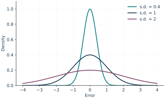
Centered Normal densities with standard deviations $0.4,1,2$ $0.4,1,2$ , on shared axes. Each has total area one; the smaller scale concentrates more probability near zero.

If $\sigma_n\to0$ $\sigma_n\to0$ , the probability $\PR(|X_n|>\varepsilon)$ $\mathbb{P}(|X_n|>\varepsilon)$ tends to zero: for nonzero scales it equals $\PR(|Z|>\varepsilon/\sigma_n)$ $\mathbb{P}(|Z|>\varepsilon/\sigma_n)$ , and for zero scales it is zero. If $\sigma_n\to\infty$ $\sigma_n\to\infty$ , then for every fixed $M>0$ $M>0$ , $\PR(|X_n|>M)=\PR(|Z|>M/\sigma_n)\to1$ $\mathbb{P}(|X_n|>M)=\mathbb{P}(|Z|>M/\sigma_n)\to1$ , since $\PR(Z=0)=0$ $\mathbb{P}(Z=0)=0$ . This contradicts the definition of $O_P(1)$ $O_P(1)$ , for example with $\eta=1/2$ $\eta=1/2$ . All arguments use marginal probabilities only.

High priorityConsistency from a stochastic rate

Exercise 2#

Prove that $a_n(T_n-\nu)=O_P(1)$ $a_n(T_n-\nu)=O_P(1)$ with deterministic $a_n\to\infty$ $a_n\to\infty$ implies $T_n\xrightarrow{P}\nu$ $T_n\overset{P}{\longrightarrow}\nu$ .

Reveal solution

Fix $\varepsilon,\eta>0$ $\varepsilon,\eta>0$ . Choose $M,N$ $M,N$ so that $\PR(a_n\|T_n-\nu\|>M)<\eta$ $\mathbb{P}(a_n\|T_n-\nu\|>M)<\eta$ for $n\ge N$ $n\ge N$ . Eventually $a_n\varepsilon\ge M$ $a_n\varepsilon\ge M$ , and then \[\PR(\|T_n-\nu\|>\varepsilon) \le\PR(a_n\|T_n-\nu\|>M)<\eta.\] $\mathbb{P}(\|T_n-\nu\|>\varepsilon) \le\mathbb{P}(a_n\|T_n-\nu\|>M)<\eta.$ Since $\eta$ $\eta$ is arbitrary, the probability tends to zero. In a statistical model this proof is applied under each fixed $P$ $P$ , with constants that may depend on $P$ $P$ .

High priorityWeak law under a finite first absolute moment

Exercise 3#

Derive Theorem 4 from the truncation theorem when $\E|X_1|<\infty$ $\mathbb{E}|X_1|<\infty$ .

Reveal solution

The variables $|X_1|\mathbf 1_{\{|X_1|>n\}}$ $|X_1|\mathbf 1_{\{|X_1|>n\}}$ tend pointwise to zero and are dominated by the integrable variable $|X_1|$ $|X_1|$ . Hence \[n\PR(|X_1|>n) \le\E[|X_1|\mathbf 1_{\{|X_1|>n\}}]\to0.\] $n\mathbb{P}(|X_1|>n) \le\mathbb{E}[|X_1|\mathbf 1_{\{|X_1|>n\}}]\to0.$ Also $X_1\mathbf 1_{\{|X_1|\le n\}}\to X_1$ $X_1\mathbf 1_{\{|X_1|\le n\}}\to X_1$ pointwise, with the same absolute dominator, so $a_n\to\mu=\E X_1$ $a_n\to\mu=\mathbb{E}X_1$ . Both applications of dominated convergence use one fixed $X_1$ $X_1$ , not an unproved pathwise limit of the moving observations $X_n$ $X_n$ . For large $n$ $n$ , $|a_n-\mu|\le\varepsilon/2$ $|a_n-\mu|\le\varepsilon/2$ , so Theorem 3 gives $\PR(|\bar X_n-\mu|>\varepsilon) \le\PR(|\bar X_n-a_n|>\varepsilon/2)\to0$ $\mathbb{P}(|\bar X_n-\mu|>\varepsilon) \le\mathbb{P}(|\bar X_n-a_n|>\varepsilon/2)\to0$ .

Mid priorityConsistency of sample variance

Exercise 4#

For i.i.d. $X_i$ $X_i$ with $\E X_1^2<\infty$ $\mathbb{E}X_1^2<\infty$ , show that $V_n$ $V_n$ and $S_n^2$ $S_n^2$ from the main prompt converge in probability to $\Var(X_1)$ $\mathrm{Var}(X_1)$ .

Reveal solution

Finite second moment implies a finite first absolute moment. Apply the weak LLN to $X_i$ $X_i$ and separately to $X_i^2$ $X_i^2$ : \[\bar X_n\xrightarrow{P}\mu,\qquad \frac1n\sum_iX_i^2\xrightarrow{P}\E X_1^2.\] $\bar X_n\overset{P}{\longrightarrow}\mu,\qquad \frac1n\sum_iX_i^2\overset{P}{\longrightarrow}\mathbb{E}X_1^2.$ The vector of these two quantities converges in probability by the union bound. Continuity of $(u,v)\mapsto v-u^2$ $(u,v)\mapsto v-u^2$ gives \[V_n=\frac1n\sum_iX_i^2-\bar X_n^2 \xrightarrow{P}\E X_1^2-\mu^2=\Var(X_1).\] $V_n=\frac1n\sum_iX_i^2-\bar X_n^2 \overset{P}{\longrightarrow}\mathbb{E}X_1^2-\mu^2=\mathrm{Var}(X_1).$ Finally $S_n^2=\frac n{n-1}V_n$ $S_n^2=\frac n{n-1}V_n$ for $n\ge2$ $n\ge2$ , and $n/(n-1)\to1$ $n/(n-1)\to1$ . Joint convergence with that deterministic factor and continuity of multiplication prove the second claim. No fourth moment was used.

Low priority — not examined: Consistency and rate of the uniform maximum

Exercise 5#

For i.i.d. Uniform$[0,\theta]$ $[0,\theta]$ data with $\theta>0$ $\theta>0$ , prove consistency and $n$ $n$ -consistency of $M_n=\max_iX_i$ $M_n=\max_iX_i$ by computing its error tails.

Reveal solution

For $0\le x\le\theta$ $0\le x\le\theta$ , independence gives $\PR(M_n\le x)=(x/\theta)^n$ $\mathbb{P}(M_n\le x)=(x/\theta)^n$ . The distribution is continuous, so strict versus nonstrict inequalities at a fixed $x$ $x$ give the same result. For $0<\varepsilon<\theta$ $0<\varepsilon<\theta$ , \[\PR(|M_n-\theta|>\varepsilon) =\left(1-\frac\varepsilon\theta\right)^n\to0;\] $\mathbb{P}(|M_n-\theta|>\varepsilon) =\left(1-\frac\varepsilon\theta\right)^n\to0;$ for $\varepsilon\ge\theta$ $\varepsilon\ge\theta$ the probability is zero. Thus $M_n$ $M_n$ is consistent. For $0\le t\le n\theta$ $0\le t\le n\theta$ , \[\PR(n|M_n-\theta|>t) =\left(1-\frac{t}{n\theta}\right)^n\le e^{-t/\theta},\] $\mathbb{P}(n|M_n-\theta|>t) =\left(1-\frac{t}{n\theta}\right)^n\le e^{-t/\theta},$ and for $t>n\theta$ $t>n\theta$ the probability is zero. The exponential bound holds uniformly over $n$ $n$ . Choosing $t$ $t$ large enough makes it less than any given $\eta>0$ $\eta>0$ , proving $n(M_n-\theta)=O_P(1)$ $n(M_n-\theta)=O_P(1)$ . The sign of $M_n-\theta$ $M_n-\theta$ is nonpositive; the absolute error was used only to state its magnitude.

Mid priorityProduct rule for stochastic orders

Exercise 6#

Prove $o_P(1)\subset O_P(1)$ $o_P(1)\subset O_P(1)$ and that $U_n=o_P(1)$ $U_n=o_P(1)$ , $V_n=O_P(1)$ $V_n=O_P(1)$ imply $U_nV_n=o_P(1)$ $U_nV_n=o_P(1)$ , without independence.

Reveal solution

If $U_n\xrightarrow{P}0$ $U_n\overset{P}{\longrightarrow}0$ , then for each $\eta>0$ $\eta>0$ we eventually have $\PR(|U_n|>1)<\eta$ $\mathbb{P}(|U_n|>1)<\eta$ , which proves $O_P(1)$ $O_P(1)$ using $M=1$ $M=1$ . For the product, fix $\varepsilon,\eta>0$ $\varepsilon,\eta>0$ and choose $M>0$ $M>0$ so that $\PR(|V_n|>M)<\eta/2$ $\mathbb{P}(|V_n|>M)<\eta/2$ eventually. The event inclusion \[\{|U_nV_n|>\varepsilon\} \subset\{|V_n|>M\}\cup\{|U_n|>\varepsilon/M\}\] $\{|U_nV_n|>\varepsilon\} \subset\{|V_n|>M\}\cup\{|U_n|>\varepsilon/M\}$ gives a probability bound below $\eta$ $\eta$ for all sufficiently large $n$ $n$ . No factorization of probabilities was used. Dividing by deterministic positive scales gives the general product rule in the main text.

High priorityConvergence in probability without almost-sure convergence

Exercise 7#

Let $B_n$ $B_n$ , $n\ge2$ $n\ge2$ , be independent Bernoulli variables with $\PR(B_n=1)=1/n$ $\mathbb{P}(B_n=1)=1/n$ . Show that $B_n\xrightarrow{P}0$ $B_n\overset{P}{\longrightarrow}0$ , but almost surely $B_n=1$ $B_n=1$ for infinitely many $n$ $n$ .

Reveal solution

For $0<\varepsilon<1$ $0<\varepsilon<1$ , $\PR(|B_n|>\varepsilon)=1/n\to0$ $\mathbb{P}(|B_n|>\varepsilon)=1/n\to0$ ; for $\varepsilon\ge1$ $\varepsilon\ge1$ the probability is zero. For fixed $N\ge2$ $N\ge2$ , \[\PR(B_N=\cdots=B_m=0) =\prod_{n=N}^m(1-1/n)=\frac{N-1}{m}\to0.\] $\mathbb{P}(B_N=\cdots=B_m=0) =\prod_{n=N}^m(1-1/n)=\frac{N-1}{m}\to0.$ Continuity from above implies that the probability of all zeros after $N$ $N$ is zero. The union of these events over $N$ $N$ still has probability zero. Its complement is the event of infinitely many ones. On that event $B_n$ $B_n$ does not tend to zero, proving the claimed distinction.

High priorityBorel–Cantelli via the expected number of occurrences

Exercise 8#

Give a second proof of the first Borel–Cantelli lemma using $N=\sum_{n\ge1}\mathbf 1_{E_n}$ $N=\sum_{n\ge1}\mathbf 1_{E_n}$ and nonnegative integration.

Reveal solution

Monotone convergence (equivalently Tonelli for a nonnegative sum) gives $\E N=\sum_n\PR(E_n)<\infty$ $\mathbb{E}N=\sum_n\mathbb{P}(E_n)<\infty$ . Markov’s inequality implies $\PR(N\ge K)\le\E N/K$ $\mathbb{P}(N\ge K)\le\mathbb{E}N/K$ for each $K>0$ $K>0$ ; hence $\PR(N=\infty)=0$ $\mathbb{P}(N=\infty)=0$ . Only finitely many of the events occur a.s. For convergence of errors, apply this result at each tolerance $1/m$ $1/m$ and intersect countably many probability-one events. An uncountable intersection is unnecessary.

Mid priorityPareto distribution: finite mean and infinite variance

Exercise 9#

Let $X\ge1$ $X\ge1$ have tail $\PR(X>t)=t^{-\alpha}$ $\mathbb{P}(X>t)=t^{-\alpha}$ for $t\ge1$ $t\ge1$ , with $1<\alpha<2$ $1<\alpha<2$ . Calculate its first and second moments and explain which weak LLN applies to i.i.d. copies.

Reveal solution

The tail-integral formulas give \[\E X=\int_0^1 1\,dt+\int_1^\infty t^{-\alpha}\,dt =1+\frac1{\alpha-1}=\frac\alpha{\alpha-1}<\infty,\] $\mathbb{E}X=\int_0^1 1\,dt+\int_1^\infty t^{-\alpha}\,dt =1+\frac1{\alpha-1}=\frac\alpha{\alpha-1}<\infty,$ while \[\E X^2=2\int_0^1t\,dt+2\int_1^\infty t^{1-\alpha}\,dt=\infty.\] $\mathbb{E}X^2=2\int_0^1t\,dt+2\int_1^\infty t^{1-\alpha}\,dt=\infty.$ The variance bound in Theorem 1 is unavailable. Theorem 4 does apply, so the sample mean converges in probability to $\alpha/(\alpha-1)$ $\alpha/(\alpha-1)$ . That theorem supplies consistency, not a $\sqrt n$ $\sqrt n$ rate for this example.

Low priority — not examined: Proof of the weighted strong law

Exercise 10#

Prove Theorem 6 by truncation, geometric subsequences, and Borel–Cantelli.

Reveal solution

First suppose $X_i=Z_i\ge0$ $X_i=Z_i\ge0$ , with $\mu=\E Z_1<\infty$ $\mu=\mathbb{E}Z_1<\infty$ . Put $Y_i=Z_i\mathbf 1_{\{Z_i\le i\}}$ $Y_i=Z_i\mathbf 1_{\{Z_i\le i\}}$ and $R_n=\sum_{i=1}^n c_iY_i$ $R_n=\sum_{i=1}^n c_iY_i$ . Since $\sum_{i\ge1}\PR(Z_i>i)\le\int_0^\infty\PR(Z_1>t)\,dt=\mu$ $\sum_{i\ge1}\mathbb{P}(Z_i>i)\le\int_0^\infty\mathbb{P}(Z_1>t)\,dt=\mu$ , the first Borel–Cantelli lemma gives $Y_i=Z_i$ $Y_i=Z_i$ eventually a.s. Their weighted partial sums therefore differ by a finite random quantity for all sufficiently large $n$ $n$ .

Summability along geometric subsequences.

Tonelli and $\sum_{i\ge k}i^{-2}\le2/k$ $\sum_{i\ge k}i^{-2}\le2/k$ for $k\ge1$ $k\ge1$ imply \[\sum_{i\ge1}\frac{\E[Z_1^2\mathbf 1_{\{Z_1\le i\}}]}{i^2} =\E\left[Z_1^2\sum_{i\ge\max(1,\lceil Z_1\rceil)}\frac1{i^2}\right] \le2\E Z_1<\infty.\] $\sum_{i\ge1}\frac{\mathbb{E}[Z_1^2\mathbf 1_{\{Z_1\le i\}}]}{i^2} =\mathbb{E}\left[Z_1^2\sum_{i\ge\max(1,\lceil Z_1\rceil)}\frac1{i^2}\right] \le2\mathbb{E}Z_1<\infty.$ For $0\le Z_1\le1$ $0\le Z_1\le1$ use $Z_1^2\le Z_1$ $Z_1^2\le Z_1$ ; for $Z_1>1$ $Z_1>1$ use $\lceil Z_1\rceil\ge Z_1$ $\lceil Z_1\rceil\ge Z_1$ in the bound. Fix $\alpha>1$ $\alpha>1$ and $k_m=\lfloor\alpha^m\rfloor$ $k_m=\lfloor\alpha^m\rfloor$ . Ignore the finitely many initial repeated indices. There is a constant $K_\alpha<\infty$ $K_\alpha<\infty$ such that $\sum_{m:k_m\ge i}k_m^{-2}\le K_\alpha/i^2$ $\sum_{m:k_m\ge i}k_m^{-2}\le K_\alpha/i^2$ : for large $m$ $m$ , $k_m\ge\alpha^m/2$ $k_m\ge\alpha^m/2$ , and summing the geometric series from the first $m$ $m$ with $k_m\ge i$ $k_m\ge i$ proves the bound, enlarging the constant for small indices. Independence and $c_i\le C$ $c_i\le C$ now yield

\[\begin{split} \sum_m\PR(|R_{k_m}-\E R_{k_m}|>\varepsilon k_m) &\le\frac{C^2}{\varepsilon^2} \sum_i\E Y_i^2\sum_{m:k_m\ge i}\frac1{k_m^2}\\ &\le\frac{C^2K_\alpha}{\varepsilon^2} \sum_i\frac{\E Y_i^2}{i^2}<\infty. \end{split}\] $\begin{split} \sum_m\mathbb{P}(|R_{k_m}-\mathbb{E}R_{k_m}|>\varepsilon k_m) &\le\frac{C^2}{\varepsilon^2} \sum_i\mathbb{E}Y_i^2\sum_{m:k_m\ge i}\frac1{k_m^2}\\ &\le\frac{C^2K_\alpha}{\varepsilon^2} \sum_i\frac{\mathbb{E}Y_i^2}{i^2}<\infty. \end{split}$

(5)

Apply Borel–Cantelli at $\varepsilon=1,1/2,1/3,\ldots$ $\varepsilon=1,1/2,1/3,\ldots$ to obtain $(R_{k_m}-\E R_{k_m})/k_m\to0$ $(R_{k_m}-\mathbb{E}R_{k_m})/k_m\to0$ a.s.

Extension from subsequences to the full sequence.

Both $R_n$ $R_n$ and $\E R_n$ $\mathbb{E}R_n$ are nondecreasing. For $k_m\le n<k_{m+1}$ $k_m\le n<k_{m+1}$ , \[\begin{split} R_n-\E R_n &\le R_{k_{m+1}}-\E R_{k_{m+1}} +\E R_{k_{m+1}}-\E R_{k_m},\\ R_n-\E R_n &\ge R_{k_m}-\E R_{k_m} -(\E R_{k_{m+1}}-\E R_{k_m}). \end{split}\] $\begin{split} R_n-\mathbb{E}R_n &\le R_{k_{m+1}}-\mathbb{E}R_{k_{m+1}} +\mathbb{E}R_{k_{m+1}}-\mathbb{E}R_{k_m},\\ R_n-\mathbb{E}R_n &\ge R_{k_m}-\mathbb{E}R_{k_m} -(\mathbb{E}R_{k_{m+1}}-\mathbb{E}R_{k_m}). \end{split}$ The expectation increment is at most $C\mu(k_{m+1}-k_m)$ $C\mu(k_{m+1}-k_m)$ . Divide by $n\ge k_m$ $n\ge k_m$ and use $k_{m+1}/k_m\to\alpha$ $k_{m+1}/k_m\to\alpha$ to conclude $\limsup_n|R_n-\E R_n|/n\le C\mu(\alpha-1)$ $\limsup_n|R_n-\mathbb{E}R_n|/n\le C\mu(\alpha-1)$ a.s. Intersect these probability-one events for $\alpha=1+1/j$ $\alpha=1+1/j$ , $j\ge1$ $j\ge1$ , and let $j\to\infty$ $j\to\infty$ . Thus $(R_n-\E R_n)/n\to0$ $(R_n-\mathbb{E}R_n)/n\to0$ a.s.

Truncation bias and recovery of the original sums.

Dominated convergence gives $\E Y_i\to\mu$ $\mathbb{E}Y_i\to\mu$ . Consequently \[\left|\frac1n\sum_{i=1}^n c_i(\E Y_i-\mu)\right| \le\frac Cn\sum_{i=1}^n|\E Y_i-\mu|\to0.\] $\left|\frac1n\sum_{i=1}^n c_i(\mathbb{E}Y_i-\mu)\right| \le\frac Cn\sum_{i=1}^n|\mathbb{E}Y_i-\mu|\to0.$ The last step is the elementary Cesàro fact: the averages of a convergent-to-zero sequence tend to zero, proved by splitting off a fixed finite initial segment. Combining the centered limit, this bias bound, and eventual equality of $Y_i,Z_i$ $Y_i,Z_i$ proves the weighted theorem for nonnegative observations.

For signed $X_i$ $X_i$ , apply the established nonnegative result to the i.i.d. sequences $X_i^+$ $X_i^+$ and $X_i^-$ $X_i^-$ , both integrable. Intersect their two probability-one events and subtract. This step avoids using monotonicity for signed partial sums, which would be invalid.

Low priority — not examined: Necessity of integrability for the strong law

Exercise 11#

Suppose $X_i$ $X_i$ are i.i.d. and $n^{-1}\sum_{i=1}^nX_i$ $n^{-1}\sum_{i=1}^nX_i$ converges a.s. to a finite limit. Show that $\E|X_1|<\infty$ $\mathbb{E}|X_1|<\infty$ .

Reveal solution

Write $A_n=n^{-1}\sum_{i=1}^nX_i$ $A_n=n^{-1}\sum_{i=1}^nX_i$ . Then $X_n/n=A_n-\frac{n-1}{n}A_{n-1}\to0$ $X_n/n=A_n-\frac{n-1}{n}A_{n-1}\to0$ a.s. If $\sum_n\PR(|X_n|>n)=\infty$ $\sum_n\mathbb{P}(|X_n|>n)=\infty$ , independence would give, for each $N$ $N$ , \[\PR(|X_n|\le n\text{ for all }n\ge N) =\lim_{m\to\infty}\prod_{n=N}^m(1-\PR(|X_n|>n)) \le\lim_{m\to\infty}e^{-\sum_{n=N}^m\PR(|X_n|>n)}=0.\] $\mathbb{P}(|X_n|\le n\text{ for all }n\ge N) =\lim_{m\to\infty}\prod_{n=N}^m(1-\mathbb{P}(|X_n|>n)) \le\lim_{m\to\infty}e^{-\sum_{n=N}^m\mathbb{P}(|X_n|>n)}=0.$ Taking the countable union over $N$ $N$ contradicts $X_n/n\to0$ $X_n/n\to0$ a.s. This argument used independence for the product and identical distribution to replace $X_n$ $X_n$ by $X_1$ $X_1$ . Therefore $\sum_n\PR(|X_1|>n)<\infty$ $\sum_n\mathbb{P}(|X_1|>n)<\infty$ . Since the tail is decreasing, \[\E|X_1|=\int_0^\infty\PR(|X_1|>t)\,dt \le1+\sum_{n\ge1}\PR(|X_1|>n)<\infty.\] $\mathbb{E}|X_1|=\int_0^\infty\mathbb{P}(|X_1|>t)\,dt \le1+\sum_{n\ge1}\mathbb{P}(|X_1|>n)<\infty.$

Low priority — not examined: Glivenko–Cantelli for discontinuous distributions

Exercise 12#

Extend the continuous-CDF proof of Glivenko–Cantelli to an arbitrary CDF $F$ $F$ using its quantile function.

Reveal solution

For $0<u<1$ $0<u<1$ , let $q(u)=\inf\{x:F(x)\ge u\}$ $q(u)=\inf\{x:F(x)\ge u\}$ . Monotonicity, right-continuity, and the endpoint limits of a CDF give \[q(u)\le x\quad\Longleftrightarrow\quad u\le F(x).\] $q(u)\le x\quad\Longleftrightarrow\quad u\le F(x).$ For completeness, $u\le F(x)$ $u\le F(x)$ places $x$ $x$ in the defining set and gives $q(u)\le x$ $q(u)\le x$ . In the other direction, the set contains points arbitrarily close above $q(u)$ $q(u)$ ; right-continuity gives $F(q(u))\ge u$ $F(q(u))\ge u$ , and monotonicity then gives $F(x)\ge u$ $F(x)\ge u$ . This also proves measurability of $q$ $q$ .

Let $U_i$ $U_i$ be i.i.d. Uniform$(0,1)$ $(0,1)$ and construct $X_i'=q(U_i)$ $X_i'=q(U_i)$ . Then $X_i'$ $X_i'$ are i.i.d. with CDF $F$ $F$ . If $G_n$ $G_n$ is the empirical CDF of the $U_i$ $U_i$ , the equivalence gives \[F_n'(x)=G_n(F(x)),\qquad \sup_x|F_n'(x)-F(x)|\le\sup_{0\le u\le1}|G_n(u)-u|\to0 \quad\hbox{a.s.}\] $F_n'(x)=G_n(F(x)),\qquad \sup_x|F_n'(x)-F(x)|\le\sup_{0\le u\le1}|G_n(u)-u|\to0 \quad\text{a.s.}$ The last result is the already proved continuous-CDF case. The constructed sequence $(X_i')$ $(X_i')$ and the original i.i.d. sequence $(X_i)$ $(X_i)$ have the same joint law. The uniform-convergence event is measurable: by right-continuity, the supremum over $x\in\R$ $x\in\mathbb{R}$ equals the supremum over rational $x$ $x$ . Its probability is therefore the same for the two sequences, and equals one. Atoms cause no difficulty for this argument.

Mid priorityFailure of argmin consistency under pointwise convergence

Exercise 13#

On $\Theta=[0,2]$ $\Theta=[0,2]$ , set $Q(\theta)=\theta^2$ $Q(\theta)=\theta^2$ and, for $n\ge2$ $n\ge2$ , put $a_n=1+1/n$ $a_n=1+1/n$ and \[Q_n(\theta)=\theta^2-4\max\{1-n^3|\theta-a_n|,0\}.\] $Q_n(\theta)=\theta^2-4\max\{1-n^3|\theta-a_n|,0\}.$ Show that $Q_n$ $Q_n$ converges pointwise to $Q$ $Q$ , but any minimizers of $Q_n$ $Q_n$ converge to 1 rather than the unique minimizer 0 of $Q$ $Q$ .

Reveal solution

The perturbation is supported on $[a_n-n^{-3},a_n+n^{-3}]$ $[a_n-n^{-3},a_n+n^{-3}]$ . For each fixed $\theta\ne1$ $\theta\ne1$ , this interval eventually misses $\theta$ $\theta$ because both endpoints tend to 1. It also misses $\theta=1$ $\theta=1$ for every $n\ge2$ $n\ge2$ , since $1/n>1/n^3$ $1/n>1/n^3$ . Thus $Q_n(\theta)=Q(\theta)$ $Q_n(\theta)=Q(\theta)$ eventually for each fixed $\theta$ $\theta$ .

Continuity and compactness give a minimizer of $Q_n$ $Q_n$ . At the center $Q_n(a_n)=a_n^2-4<0$ $Q_n(a_n)=a_n^2-4<0$ , whereas outside the support $Q_n(\theta)=\theta^2\ge0$ $Q_n(\theta)=\theta^2\ge0$ . Every minimizer must lie within $n^{-3}$ $n^{-3}$ of $a_n$ $a_n$ and hence converges to 1. Nevertheless $Q$ $Q$ has its unique minimum at 0. Finally $\sup_\theta|Q_n(\theta)-Q(\theta)|=4$ $\sup_\theta|Q_n(\theta)-Q(\theta)|=4$ for every $n$ $n$ , displaying exactly the missing uniform control.

References

[1]

R. Durrett. Probability: Theory and examples. Cambridge university press. 2019.

[2]

W. K. Newey and D. McFadden. Large sample estimation and hypothesis testing. Handbook of econometrics, 4, 2111–2245. 1994.

[3]

J. Shao. Mathematical Statistics. Springer. 2003.

Terminology notes

An empirical process describes the sampling errors of a family of empirical averages, for example all errors $F_n(x)-F(x)$ $F_n(x)-F(x)$ as $x$ $x$ varies. Its theory includes bounds on these errors over the whole family.↩︎
An Edgeworth expansion adds correction terms to a leading Normal approximation using information such as skewness. Its validity requires additional assumptions; it is not an exact finite-sample formula.↩︎
An $M$ $M$ -estimator optimizes a data-dependent objective, often an average loss. Maximum likelihood and least squares are examples of this general estimation framework.↩︎

What changed

October 19, 2026 (instructor follow-up). Changed Section 7.1’s main results and linked sample-variance exercise to mid priority; retained the optional strong-consistency extension.

October 19, 2026: Corrected notation, wording and cross-references after the course-wide errata review; refreshed the linked HTML and PDF editions.

October 14, 2026. Added issue-reporting links to the webpage and PDF. The mathematics and priority assignments are unchanged in this update.

Comments

Discuss an idea or ask a public question. Include a section or exercise number when relevant. For errors in the notes or website, Report an issue.

Public comments use Disqus. Enable JavaScript to load them.

Email the instructor for a private question or if comments are unavailable.

Cutoff \(R\) $R$	\(A_1(R)\) $A_1(R)$	\(A_2(R)\) $A_2(R)$
\(1\) $1$	\(1\) $1$	\(1\) $1$
\(10\) $10$	\(3-2/\sqrt{10}\approx2.368\) $3-2/\sqrt{10}\approx2.368$	\(4\sqrt{10}-3\approx9.649\) $4\sqrt{10}-3\approx9.649$
\(100\) $100$	\(2.8\) $2.8$	\(37\) $37$

Lecture map

Learning goals

1. Exact inference and the asymptotic approach

2. Convergence in probability

2.1. Modes of stochastic convergence

2.2. Stochastic orders

3. Consistency of estimators

4. Laws of large numbers

4.1. Weak law under bounded variances

A finite mean, an infinite second moment

4.2. Truncation and a finite first moment

5. Strong laws and tail events (optional)

6. Uniform laws of large numbers (optional)

6.1. Empirical distribution functions

6.2. Uniform convergence over compact parameter spaces

7. Consistency of moment and likelihood estimators

7.1. Moments and continuous transformations

7.2. Uniform convergence and minimizer consistency

7.3. Regression and likelihood examples

8. Detailed reference

9. Further reading

Key ideas

Looking ahead

References

Terminology notes

Comments